Agribound
Agricultural field boundary delineation from satellite imagery with published segmentation models, geospatial foundation models and satellite embeddings, through one configuration and one pipeline.









Agribound runs a composite → delineation → post-processing → crop-filter → export pipeline over eleven sources (Landsat, Landsat panchromatic, Sentinel-2, HLS, NAIP and SPOT 6/7 composites on Google Earth Engine, USGS NAIP Plus, local GeoTIFFs, and Google Satellite Embedding and TESSERA embeddings) with seven engines (Delineate-Anything, Fields of The World, GeoAI Mask R-CNN, DINOv3, Prithvi-EO-2.0, embedding clustering and ensembles). Every run is seeded, cached under content-addressed names and documented by a provenance record; evaluation, tiling for HPC clusters and an optional human-confirmed agent layer are included.
Upgrading from 0.1.x
Version 1.0.0 fixes defects that affected results produced with agribound 0.1.x (for example FTW season windows, Landsat/HLS radiometry, caches that ignored the study area and year, and silent engine fallbacks). See the migration guide and the list of affected results.
How it works
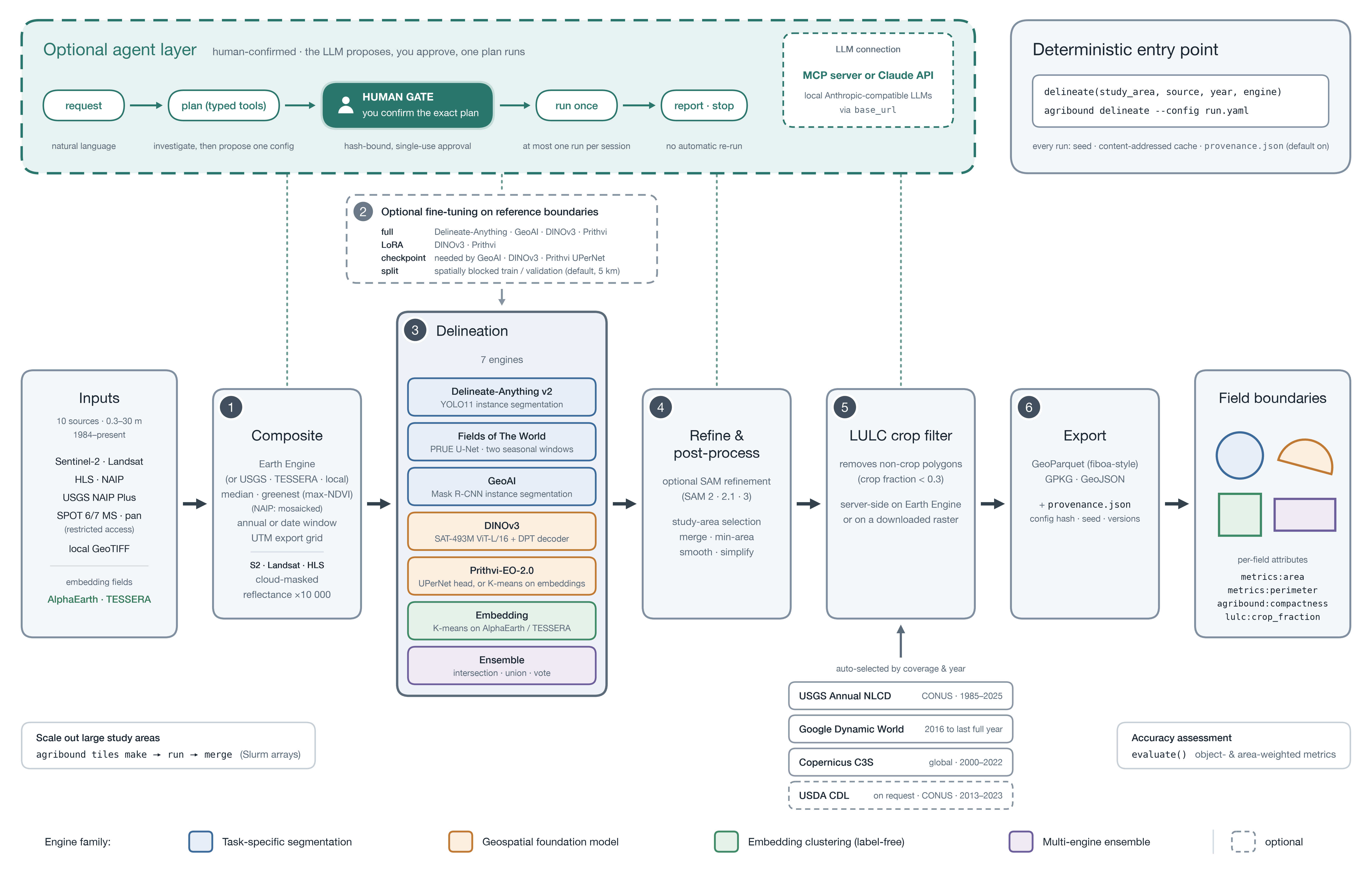
The agribound 1.0 workflow (select the image for full resolution): a six-stage pipeline from eleven imagery and embedding sources (0.3–30 m, 1984–present) to field boundaries, with a deterministic entry point and an optional, human-confirmed agent layer above it.
- Composite. Earth Engine builds a median or greenest-pixel (max-NDVI) composite for a year or a date window and exports it on a UTM grid. NAIP is mosaicked, and only Landsat, Sentinel-2 and HLS are cloud-masked and scaled to reflectance ×10 000 (Landsat panchromatic is cloud-masked but kept as TOA reflectance). USGS NAIP Plus, TESSERA and local GeoTIFF inputs are read without Earth Engine.
- Fine-tuning (optional). Full (Delineate-Anything, GeoAI, DINOv3, Prithvi) or LoRA (DINOv3, Prithvi) fine-tuning on reference boundaries, validated by default on a spatially blocked split (5 km blocks). GeoAI, DINOv3 and Prithvi's UPerNet mode need a checkpoint, from fine-tuning or supplied by the user.
- Delineation. One of seven engines, coloured by family: task-specific segmentation, geospatial foundation model, label-free embedding clustering and multi-engine ensemble.
- Refine and post-process. Optional SAM refinement (SAM 2, 2.1 or 3; the SAM 3 backends are untested), then study-area selection, merging, minimum-area filtering, smoothing and simplification.
- LULC crop filter. Removes polygons whose crop fraction is below 0.3, computed on Earth Engine or locally on a downloaded crop raster. Annual NLCD, Dynamic World or C3S Land Cover is selected by coverage and year; CDL (CONUS only) is used on request. Dynamic World files plantations and many orchards under trees, so for tree crops set
lulc_tree_crops=True, which, with Dynamic World or C3S, counts tree cover (forest included) as crop; NLCD and CDL are unchanged. - Export. GeoParquet (fiboa-style columns), GeoPackage or GeoJSON, with per-field area, perimeter, compactness and crop fraction, plus a
provenance.jsonrecord.
Around the pipeline:
- Entry point.
delineate()andagribound delineate --configrun the six stages directly. Every run is seeded and uses a content-addressed cache, andprovenance.jsonis written by default. - Agent layer (optional). A language model, reached through the Claude API or an MCP host (or a local Anthropic-compatible server via
base_url), investigates with typed read-only tools and proposes one configuration. It runs only after you confirm that exact plan at the human gate, with an approval bound to the plan's hash and used once. At most one plan runs per session, and the session then stops (see Agent layer). - Scale out and evaluate.
agribound tiles make,runandmergesplit a large study area into tiles that run as Slurm array jobs (see HPC and large areas).evaluate()scores results against reference boundaries with object-level and area-weighted metrics (see Evaluation).
Quick install
Two environments are needed for the full stack because FTW and Prithvi
require incompatible lightning versions; see Installation.
Quickstart
import agribound

gdf = agribound.delineate(
    study_area="area.geojson",
    source="sentinel2",
    year=2024,
    engine="delineate-anything",
    gee_project="my-gee-project",
)
The result is a GeoDataFrame of field polygons with area, perimeter,
compactness and provenance columns, written to fields_sentinel2_2024.gpkg
with a .provenance.json record next to it. See the
Quickstart.
LULC crop filter
Engines delineate visual boundaries, which include roads, water bodies, forest and built-up areas. The LULC filter, on by default, removes polygons whose crop fraction in a land-cover dataset is below 0.3:
- Annual NLCD (1985-2025, 30 m, classes 81/82) where at least 90 % of the area has NLCD data (conterminous US);
- otherwise Dynamic World (10 m, annual median crop probability) for 2016 up to the last complete year;
- otherwise C3S Land Cover (2000-2022, 300 m, classes 10, 11, 12, 20, 30);
- CDL (
cultivated, 2013-2023) on request.
It reads the datasets from Earth Engine for every source and raises by default when it fails. See LULC crop filter.
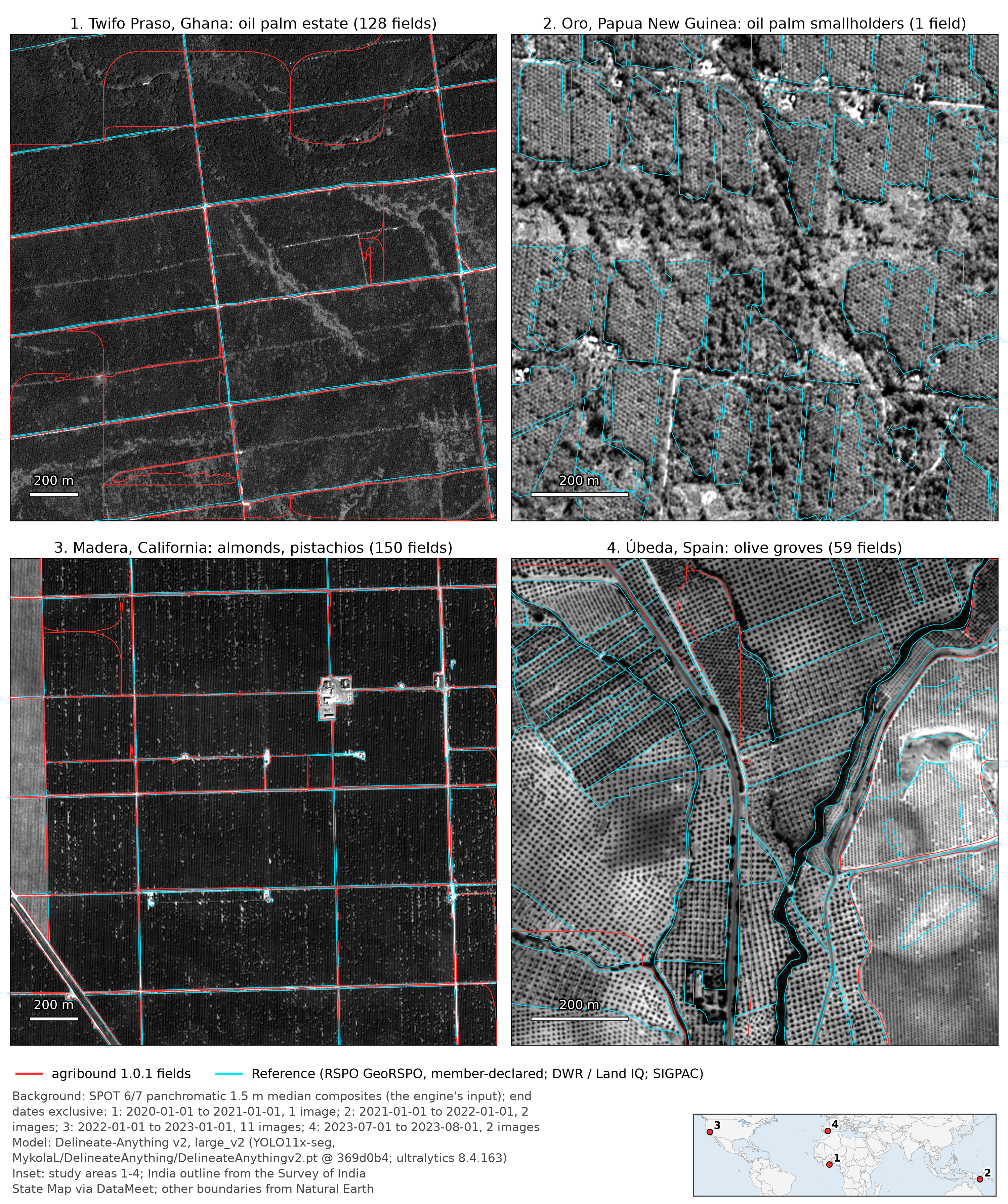
Dynamic World counts plantations and orchards as trees, so the default filter
can remove tree crops where it uses Dynamic World: of 95 oil-palm blocks in
Ghana it kept none for 2020. lulc_tree_crops=True counts tree cover as crop
and kept all 95; with Dynamic World or C3S the filter then also keeps forest
(NLCD and CDL are unchanged). See
Tree crops.
Example results
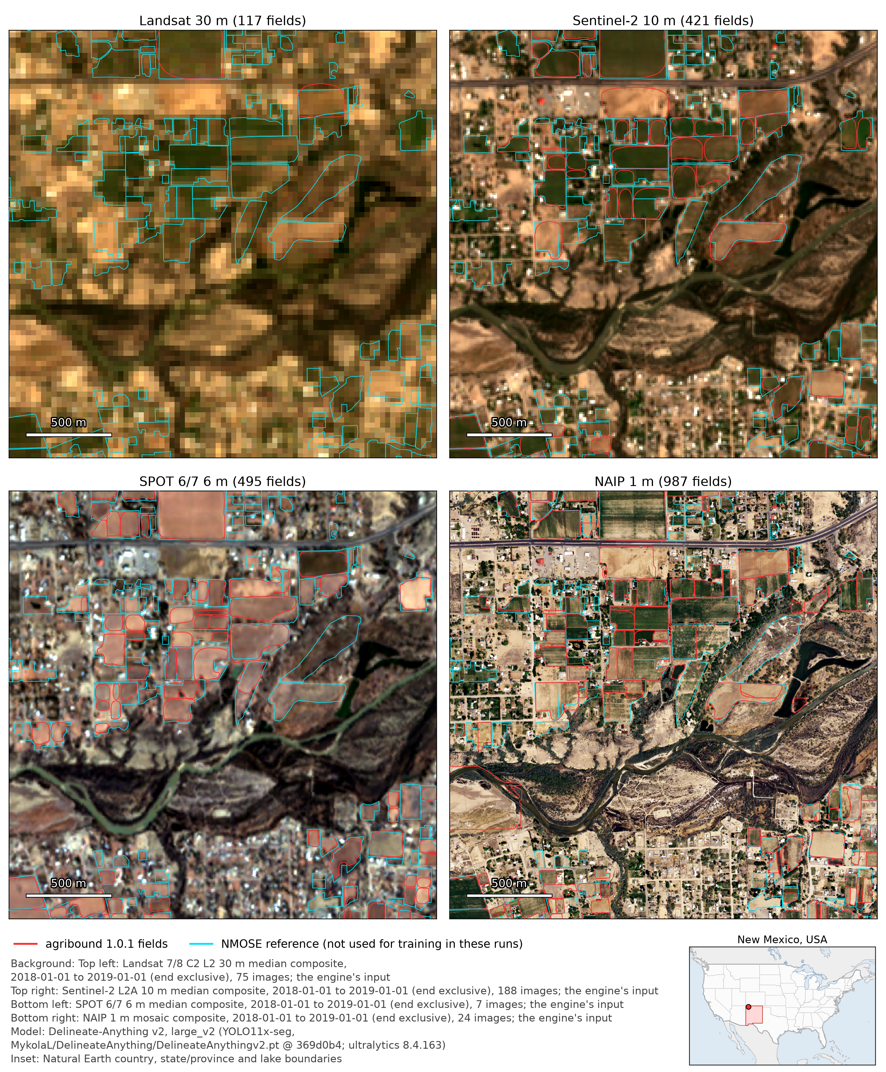
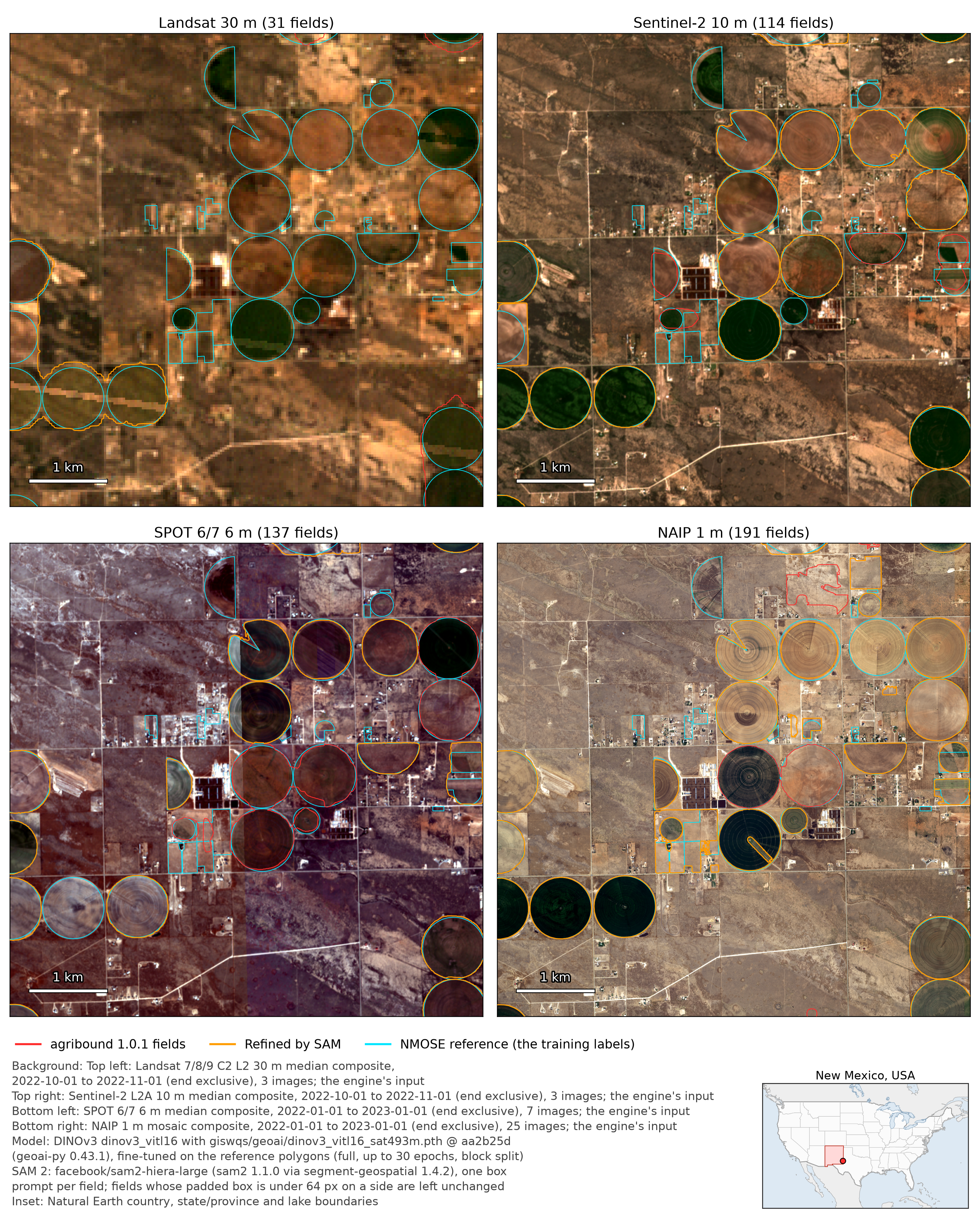
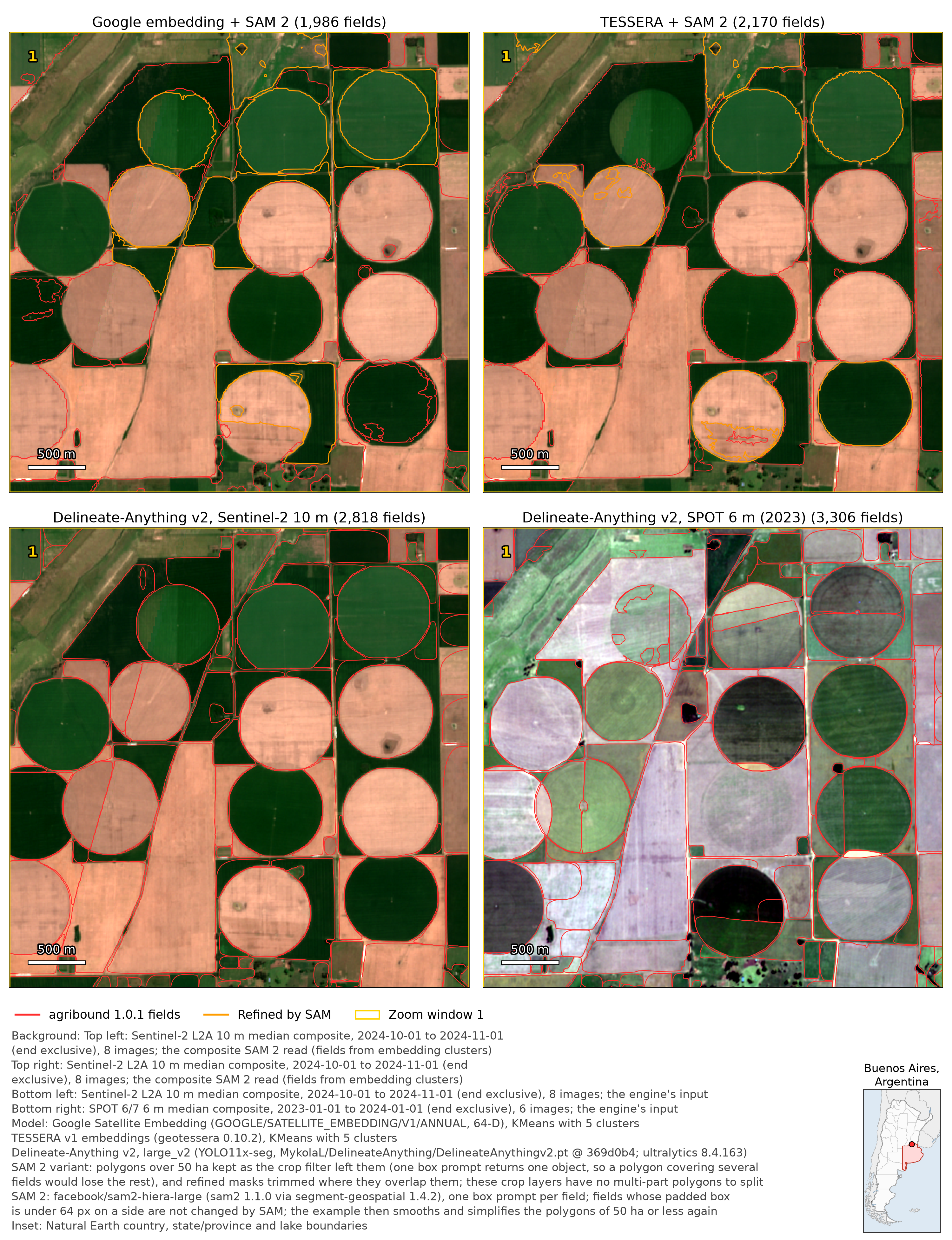
From the agribound 1.0.1 example runs (the San Juan County map shows 1.0.0 outputs, which 1.0.1 reuses unchanged; the tree-crop map comes from the development version that follows 1.0.1). Each map is drawn on a composite from the run, named under the map: usually the engine's input; for FTW, its window A; for the SAM-refined embedding panels, the Sentinel-2 composite SAM 2 read. Select an image for the full-resolution file; see the Gallery for all regions and engines.
From 30 m to 1 m (San Juan County, New Mexico). Delineate Anything v2, used as released, on Landsat, Sentinel-2, SPOT 6/7 and NAIP of 2018 against the 944 NMOSE polygons (cyan; not used for training or fine-tuning in these runs): object F1 (IoU ≥ 0.5) 0.15, 0.34, 0.33 and 0.43.
Supervised: DINOv3 fine-tuned + SAM 2 (eastern Lea County, New Mexico). In-sample F1 against the training polygons: 0.06 (Landsat), 0.38 (Sentinel-2), 0.45 (SPOT) and 0.59 (NAIP).
Label-free: embeddings + SAM 2 vs Delineate-Anything v2 (Pampas, Argentina). No reference data or training; centre pivots near Pergamino. Orange = refined by SAM 2 (parts over 50 ha kept unrefined). The embedding panels come from the agribound 1.0.1 run of 2026-09-29; the Delineate-Anything panels are the 1.0.0 outputs, which that run reused. The gallery adds the whole study area and three zoomed windows.
Tree crops (Ghana, Papua New Guinea, California, Spain). Delineate Anything
v2 as released on SPOT 6/7 panchromatic against RSPO GeoRSPO, DWR / Land IQ
and SIGPAC polygons (cyan): object F1 (IoU ≥ 0.5; precision among the
predictions that overlap a reference polygon) 0.29 for oil palm estate
blocks and one polygon among 302 oil palm smallholder parcels (68 matched after
fine-tuning on parcels of the same scheme in a square 13.6 km from the Oro
square, a run added after the released model's result there and kept after
its own score was seen); 0.86 for almond and pistachio blocks, whose fields
are in the model's training data (FBIS-73M). DINOv3, fine-tuned on the same
labels near each site (never on the evaluated squares), merges neighbouring
fields (merge rates 0.80 to 1.00). The default crop filter removes every oil
palm polygon; lulc_tree_crops=True keeps every oil palm Delineate-Anything
polygon and all but 8 of the 2,720 oil palm embedding segments. The
gallery compares the sources and engines.
Documentation
| Section | Content |
|---|---|
| Installation | environments, extras, Apple-silicon notes |
| Migrating to 1.0 | every breaking change, old vs new |
| Quickstart | Python and CLI in five minutes |
| Satellite sources | coverage, resolution, value scales, masking, LULC filter |
| Engines and SAM refinement | what each engine does, weights, parameters, limits |
| Configuration and CLI | every field and command |
| Fine-tuning | training on reference boundaries |
| Evaluation | metric definitions |
| Reproducibility | seeds, cache keys, provenance, output reuse |
| HPC and large areas | tiling, two-phase runs, Earth Engine quotas, NSF ACCESS |
| Agent layer | human-confirmed planning, MCP server |
| FTW polygon query and GEE setup | published FTW polygons by area; Earth Engine credentials and project |
| API reference | generated from the docstrings |
| Gallery | maps from the 1.0.0 and 1.0.1 example runs (example 23: the development version that follows 1.0.1) |
License
Agribound is released under the Apache 2.0 License. The Delineate-Anything model code and weights and Ultralytics are AGPL-3.0; check the licences of the models and datasets you use.