Example Gallery (agribound 1.0)
Field boundaries from the agribound example scripts, run at their default
settings. Examples 02, 05, 13, 14, 15 and 22 were re-run with agribound 1.0.1
on 2026-09-29. The other entries, except example 23's, show outputs of the
same scripts run with agribound 1.0.0 on 2026-09-28 and 29, which 1.0.1 reuses
unchanged: 1.0.1 changed only the embedding engine's clustering, SAM
refinement and output reuse, and the code paths of these entries are the same
in both releases. The 1.0.1 runs of examples 02 and 15 also reused their 1.0.0
FTW and Delineate-Anything outputs (their provenance records say 1.0.0), and
example 13's 1.0.1 output is identical to its 1.0.0 output. Example 23 was run
on 2026-10-05 (the DINOv3 comparison and the fine-tuning at Madera and Úbeda on
2026-10-06) with the development version that follows 1.0.1: it needs the
landsat-pan source with its default landsat_pan_missions rule (Landsat 8/9
only for these years), lulc_tree_crops and the corrected Delineate-Anything
fine-tuning recipe, which 1.0.1 does not have (see the changelog). Every
legend reads "agribound 1.0.1 fields", also in the images drawn from 1.0.0
outputs and in those of example 23. Example 13 refines example 20's output
(see its entry); examples 01 and 12 were not run end to end (12's NAIP runs
were). The 0.1.x screenshots are kept on the
archived 0.1.x page.
How to read the images. Red outlines are agribound output, cyan outlines are reference polygons and orange outlines are fields that SAM refined. Each map is drawn on a composite from the run, named under the map: usually the engine's input; for FTW, window A, the first of FTW's two season inputs; for the SAM entries, the composite SAM read. The imagery therefore shows the acquisition period of that composite. Zoom panels and cropped windows show the square with the most polygons of one layer (named in each entry), not a random sample of the study area; the Pampas windows (example 15) follow the rules their entries state. The number in a panel title counts every polygon in that output, not only those inside the window shown. The inset locates the study area (red dot) in its country (in example 22 and in the first and last images of example 23, the study areas, numbered as the panels, on a world map); India is drawn from the Survey of India outline, all other boundaries from Natural Earth. Under each image are the imagery, the model and its version.
SPOT colours. SPOT 6/7 multispectral composites are uncalibrated digital numbers, and each of their bands is stretched separately, while the other sources share one stretch across R, G and B. SPOT colours therefore cannot be compared with those of the other sources: bare soil often looks mauve or lavender (examples 03, 11, 14 and 15). A median of a few SPOT scenes can also show straight, sudden colour steps. The SPOT panel of example 14 (7 images) has a nearly vertical one about halfway across that shows several pivots in two tones. The step is in the composite the engine read, not added by the rendering. SPOT-Pan panels are shown in grey.
Crop filter. Unless an entry says otherwise, the polygons pass a crop filter at a threshold of 0.30: outside the conterminous US, Dynamic World (the polygon mean of the year's median crop probability); in the conterminous US, Annual NLCD (the share of cultivated-crop and pasture/hay pixels, classes 82 and 81). The minimum field area is given in each entry.
What these images show
Each image shows what one configuration produces, not how accurate it is. Accuracy is reported only where a reference layer exists (examples 12, 13, 14 and 20, all against the NMOSE polygons in New Mexico; for 14 and for the fine-tuned models of 12 they are also the training labels, so those scores are in-sample; example 23 against RSPO, DWR / Land IQ and SIGPAC polygons, with its fine-tuned models trained elsewhere; Delineate Anything v2's own training data (FBIS-73M) cover the Madera square and 87 % of the Úbeda square, so its scores there are mostly on fields it has seen).
The images are rendered at 3000 px by
tools/make_gallery.py
from the run outputs. This page shows 1600 px WebP previews; click an image to
open the full-resolution PNG. The numbers below come from the run logs, the
evaluation metrics files and
assets/gallery_1.0/gallery_stats.json.
Models and versions
| Engine | Model and version used in these runs |
|---|---|
| Delineate-Anything | Delineate Anything v2, large_v2 (YOLO11x-seg, trained on FBIS-73M): DelineateAnythingv2.pt from Hugging Face MykolaL/DelineateAnything at revision 369d0b4, SHA-256 pinned; agribound's native implementation with ultralytics 8.4.163; confidence threshold 0.15 |
| FTW | FTW_PRUE_EFNET_B5 ("FTW v3: Standard, B5": PRUE U-Net with an EfficientNet-B5 encoder), ftw-baselines v3 checkpoint, SHA-256 pinned; run with ftw-tools 2.0.0b5 (a pre-release); no fine-tuning |
| SAM 2 | facebook/sam2-hiera-large (SAM 2.0 Hiera-L, not 2.1), through segment-geospatial 1.4.2 and the sam2 1.1.0 package; one box prompt per field |
| Prithvi | ibm-nasa-geospatial/Prithvi-EO-2.0-300M-TL at revision 63adbd3, terratorch 1.2.13 |
| GeoAI | torchvision Mask R-CNN ResNet50-FPN via geoai-py 0.43.1, fine-tuned on the reference polygons (no published field weights); chips sized from the reference fields; instances split at the inference-window edges joined |
| DINOv3 | dinov3_vitl16 (ViT-L/16) with the SAT-493M weights giswqs/geoai/dinov3_vitl16_sat493m.pth at revision aa2b25d, geoai-py 0.43.1; full fine-tuning on the reference polygons (in example 23, on the labels of a training area near each study area, never on the evaluated square; no published field weights) |
| Embeddings | Google Satellite Embedding (GOOGLE/SATELLITE_EMBEDDING/V1/ANNUAL, AlphaEarth Foundations, 64-D) and TESSERA v1 (128-D, geotessera 0.10.2); PCA to 16 components, then scikit-learn KMeans with ten restarts (n_init=10); k chosen by silhouette score among 5, 10, 15, 20, 30 and 50 unless stated (in every automatic choice here the score was highest at k = 5, the smallest candidate, and smaller k were not tested). agribound 1.0.0 used MiniBatchKMeans on rasters of more than 100,000 valid pixels, as all of these are |
SAM size rule. SAM is prompted only when a field's bounding box, padded
on every side by 15 % of its size (a factor of 1.3), is at least 64 pixels
wide and 64 pixels tall. That is an unpadded box of at least about 49 pixels
on each side (64 / 1.3 ≈ 49.2): about 490 m at 10 m, 295 m at 6 m and 49 m at
1 m. Fields below that keep their geometry. With the default
sam_overlaps="trim", a refined mask cannot take area from a neighbouring
polygon. Since 1.0.1, a mask that covers less than half of its input polygon
after that trim (sam_min_coverage, default 0.5) is not used, and the polygon
keeps its input geometry.
Lea County, New Mexico — DINOv3 fine-tuned, from 30 m to 1 m
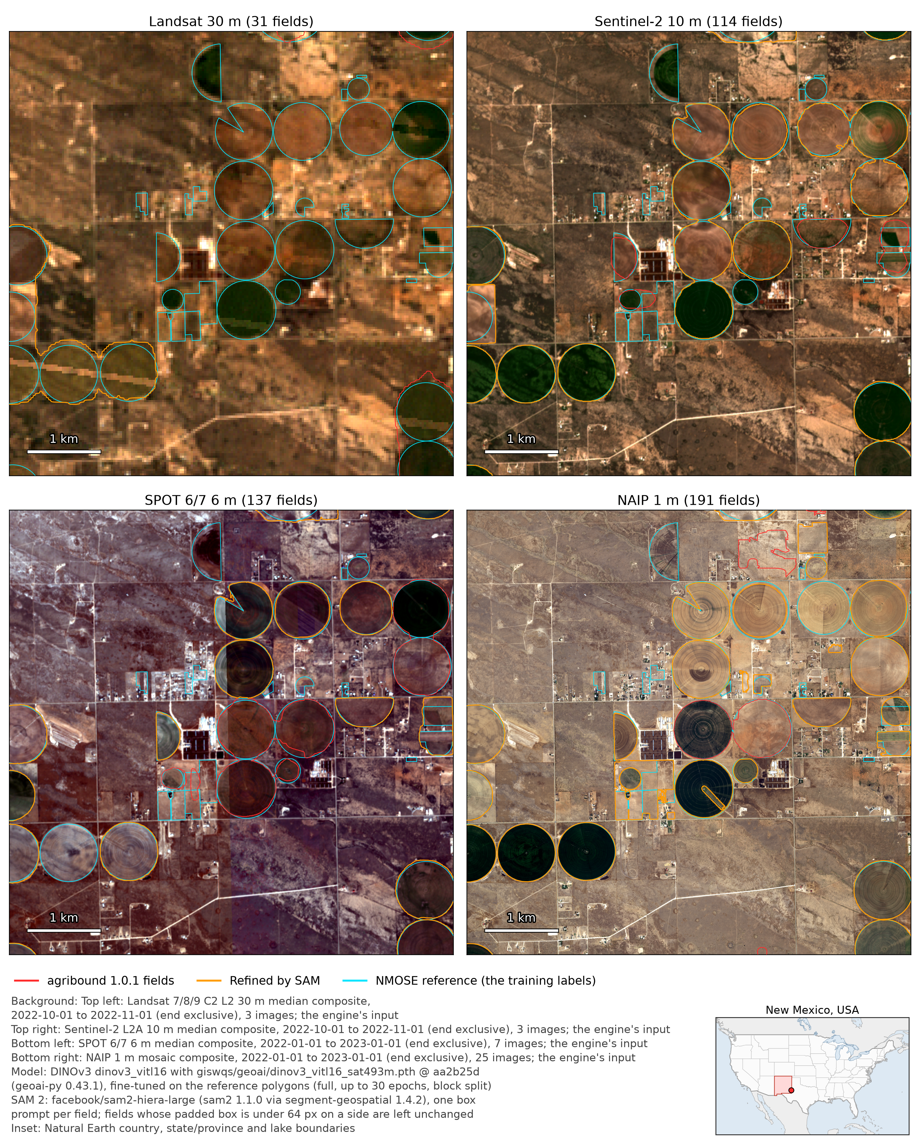
Example 14 · DINOv3 ViT-L/16 (SAT-493M weights, geoai-py 0.43.1), fully fine-tuned on the NMOSE polygons of the study area separately for each source, then refined with SAM 2 · eastern Lea County, New Mexico, north of Hobbs (the easternmost 1.3 km of the box, 7 % of its area, is in Gaines County, Texas, where NMOSE has no polygons) · 2022 · min. area 2,500 m² (5,000 m² for NAIP); Annual NLCD 2022 crop filter · window: the 6 km square with the most reference fields.
Panels: Landsat 30 m and Sentinel-2 10 m (October composites, 3 images each), SPOT 6/7 6 m (annual, 7 images; its colour step is described under "SPOT colours" above) and NAIP 1 m (25 images). The NMOSE polygons (cyan) are also the training labels, so these scores are in-sample, not an independent accuracy estimate. Against the 227 NMOSE polygons in the box (one-to-one matching at IoU ≥ 0.5), the fields and the in-sample F1 without and with SAM 2 are:
| Source | Fields (without / with SAM 2) | In-sample F1 without SAM 2 | In-sample F1 with SAM 2 |
|---|---|---|---|
| Landsat 30 m | 31 / 31 | 0.06 | 0.06 |
| Sentinel-2 10 m | 116 / 114 | 0.38 | 0.38 |
| SPOT 6/7 6 m | 137 / 137 | 0.42 | 0.45 |
| NAIP 1 m | 190 / 191 | 0.60 | 0.59 |
(HLS 30 m, not shown: in-sample F1 0.11 with and without SAM 2.) The training
data change with resolution as well: the box holds 4 training chips of 256
pixels at 30 m (3 for training, 1 for validation), 49 at 10 m, 126 at 6 m and
2,014 at 1 m, so this comparison changes the amount of training data along
with the pixel size (and NAIP uses a minimum area of 5,000 m² rather than
2,500 m²). In-sample F1 rises most with SAM 2 at 6 m (0.42 to 0.45); at 1 m
SAM 2 raises the mean IoU of matched fields from 0.88 to 0.89, while in-sample
F1 falls from 0.604 to 0.589 (126 and 123 matched fields). Many NAIP polygons
hold more than one reference field: SAM 2 was prompted with 1,164 of them and
its mask covered less than half of 463, which keep their DINOv3 outline
(sam_min_coverage, new in 1.0.1; 3, 4, 1 and 9 for Sentinel-2, Landsat, HLS
and SPOT). Run with agribound 1.0.1 on 2026-09-29; the four fine-tuned
checkpoints were trained again for it, since the fine-tuning cache key changed
before the 1.0.0 release, and the scores without SAM 2 are unchanged to two
decimals.
Lea County, New Mexico — Delineate-Anything v2, GeoAI and DINOv3 on NAIP 1 m
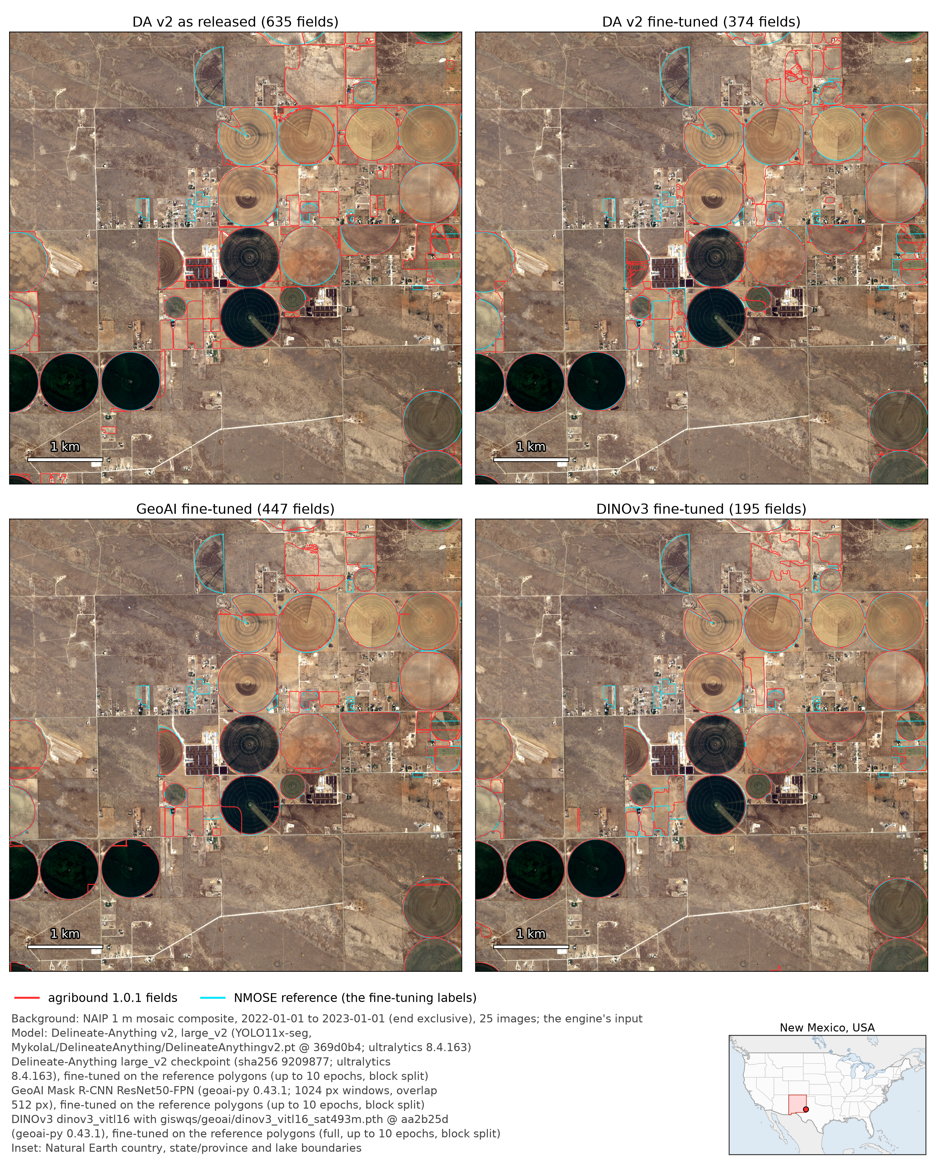
Example 12 (NAIP runs only; the rest of example 12 was not run for 1.0.0) · eastern Lea County, New Mexico, north of Hobbs (the box of example 14) · NAIP 1 m, 2022 (25 images) · min. area 5,000 m²; Annual NLCD 2022 crop filter · window: the 6 km square with the most reference fields.
Delineate Anything v2 as released (top left; a run with example 12's
settings that example 12 itself does not include) and three models
fine-tuned on the 230 NMOSE polygons of the box with example 12's settings
(10 epochs, 5 km block split): Delineate Anything v2 large_v2 (650 chips of
512 px), GeoAI Mask R-CNN (229 chips of 1,024 px) and DINOv3 (2,014 chips of
256 px). The NMOSE polygons (cyan) are the fine-tuning labels, so the scores of
the fine-tuned models are in-sample, not independent accuracy estimates.
Against the 227 NMOSE polygons in the box (one-to-one matching at IoU ≥ 0.5):
| Model | Fields | Precision | Recall | F1 | Mean IoU of matched fields | Predictions overlapping no reference polygon |
|---|---|---|---|---|---|---|
| Delineate Anything v2 as released | 635 | 0.23 | 0.64 | 0.34 | 0.86 | 261 |
| Delineate Anything v2 fine-tuned (in-sample) | 374 | 0.35 | 0.58 | 0.44 | 0.85 | 86 |
| GeoAI fine-tuned (in-sample) | 447 | 0.36 | 0.72 | 0.48 | 0.84 | 135 |
| DINOv3 fine-tuned (in-sample) | 195 | 0.64 | 0.55 | 0.59 | 0.90 | 53 |
Many of the predictions that overlap no reference polygon are fields the registry does not include (NMOSE has no polygons in the Texas strip of the box). Fine-tuning mainly reduced Delineate Anything v2's predictions outside the registry (261 to 86) at a small cost in recall.
GeoAI needed two engine changes before it produced whole fields; both are in
1.0.0. With the earlier fixed 256 px chips, every GeoAI polygon was at most one
256 m inference window (the pivots here are about 800 m across), and in-sample
F1 was 0.01 (2,902 polygons). Chips sized from the reference fields (the
1.0.0 default, here 1,024 px, 1 km; engine_params["chip_size"] overrides)
raised F1 to 0.25 (723 polygons), with straight cuts left where a field
crossed the edges of the overlapping inference windows. Joining the pieces
split at those edges (engine_params["merge_window_seams"], on by default:
448 instances joined, gaps of up to 2 px along the edges filled) gave the
result shown (F1 0.48). A few short cuts remain.
San Juan County, New Mexico — Delineate-Anything v2 from 30 m to 1 m
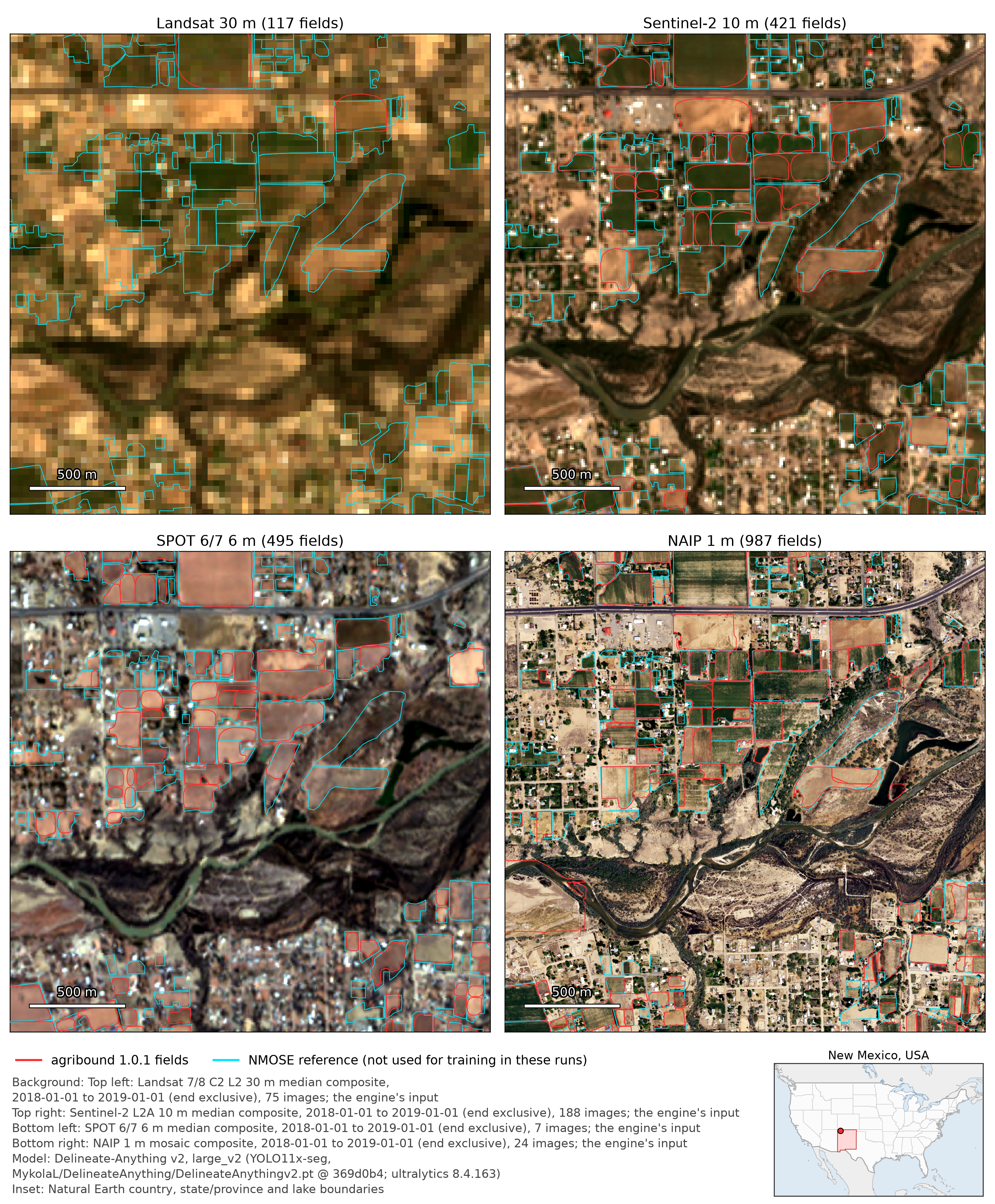
Example 20 (resolution comparison) · Delineate Anything v2 used as released, on Landsat 7/8 (a median of the Landsat 7 and 8 Collection 2 Level-2 collections; 30 m, 75 images), Sentinel-2 (10 m, 188 images), SPOT 6/7 (6 m, 7 images) and NAIP (1 m, 24 images), all 2018 annual composites · the study area of example 20 · min. area 2,500 m²; Annual NLCD 2018 crop filter · window: the 2.5 km square with the most reference fields.
2018 is the year closest to the reference's 2016 imagery that all four sources cover (NAIP is flown every two years here). Against the 944 NMOSE polygons (one-to-one matching at IoU ≥ 0.5; the polygons were not used for training or fine-tuning in these runs):
| Source | Fields in the box | Precision | Recall | F1 | Boundary F1 (10 m) |
|---|---|---|---|---|---|
| Landsat 30 m | 116 | 0.68 | 0.08 | 0.15 | 0.14 |
| Sentinel-2 10 m | 420 | 0.55 | 0.24 | 0.34 | 0.41 |
| SPOT 6/7 6 m | 494 | 0.48 | 0.25 | 0.33 | 0.43 |
| NAIP 1 m | 986 | 0.42 | 0.44 | 0.43 | 0.59 |
(Fields in the box: the predictions whose representative point lies inside the evaluation box, as in the crop-filter table below. The panel titles count each whole output, 117, 421, 495 and 987 polygons: in each run one polygon lies across the box's south edge (the west edge for NAIP), with its representative point just outside.)
Recall rises about fivefold from 30 m to 1 m and boundary F1 about fourfold; SPOT at 6 m is within 0.01 of Sentinel-2 on object F1 (0.33 and 0.34) and slightly higher on boundary F1 (0.43 and 0.41). Landsat is outside Delineate Anything v2's 0.25–10 m training range (agribound warns and records it). The crop filter removed 43 % of the output polygons on Landsat (it kept 117 of 204), 41 % on Sentinel-2 (421 of 713), 50 % on SPOT (495 of 996) and 64 % on NAIP (987 of 2,709). The reference was digitised from 2016 NAIP, so changes by 2018 count as errors.
San Juan County, New Mexico — FTW and Delineate-Anything v2 with and without the crop filter
Example 20 (crop-filter comparison) · the pre-trained FTW
(FTW_PRUE_EFNET_B5; windows 11 Mar–10 May 2019, 22 images, shown in the top
panels, and 20 Sep–19 Nov 2019, 37 images) and Delineate Anything v2 (annual
2019 composite, 171 images, bottom), both used as released, each with the
Annual NLCD 2019 crop filter on (left) and off (right) · min. area 2,500 m² ·
window: the 3 km square with the most reference fields.
With the filter off, the polygons it would remove are outlined in magenta. The filter kept 414 of FTW's 1,377 polygons and 380 of Delineate Anything v2's 562. Against the 944 NMOSE polygons (one-to-one matching at IoU ≥ 0.5; the polygons were not used for training or fine-tuning in these runs):
| Engine | Crop filter | Fields | Precision | Recall | F1 | Predictions overlapping no reference polygon |
|---|---|---|---|---|---|---|
| FTW | on | 414 | 0.39 | 0.17 | 0.24 | 63 |
| FTW | off | 1,377 | 0.12 | 0.18 | 0.15 | 976 |
| Delineate Anything v2 | on | 379 | 0.58 | 0.23 | 0.33 | 12 |
| Delineate Anything v2 | off | 561 | 0.40 | 0.24 | 0.30 | 174 |
(Fields in the box, by representative point.) Of the 963 polygons the filter removes from FTW's output, 913 overlap no reference polygon (162 of 182 for Delineate Anything v2); in this window they are mostly in the riparian strip along the river and in the built-up area. For both engines the filter raises precision and lowers recall by less than 0.01. It also removes some polygons that do overlap reference fields (a few are visible here).

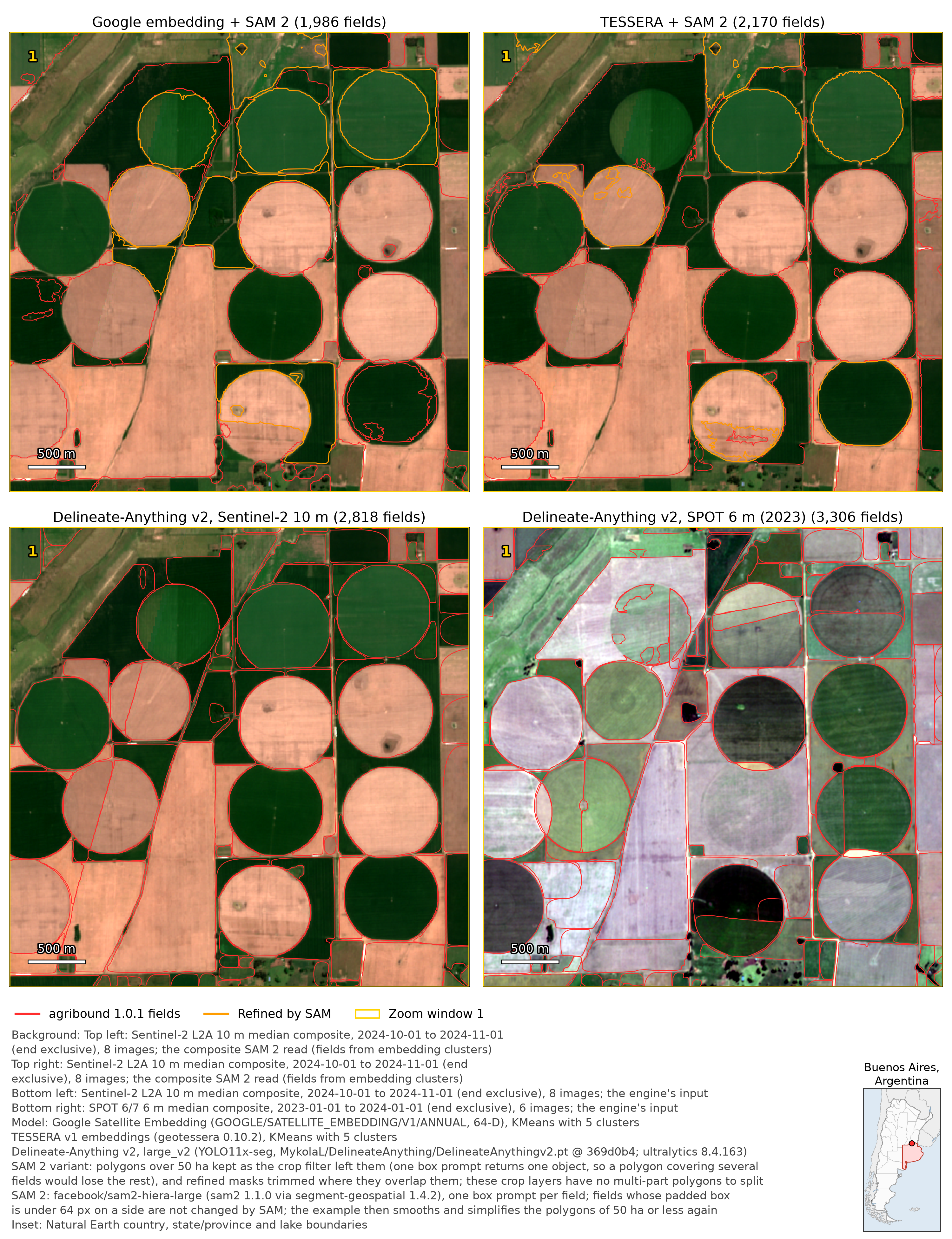
Pampas, Argentina — embeddings + SAM 2 vs Delineate-Anything v2 on Sentinel-2 and SPOT
Example 15 · Pergamino partido, Buenos Aires Province, east of the city · label-free (no training and no reference data) · min. area 5,000 m²; Dynamic World crop filter of each input's year (2024; 2023 for SPOT) · window: zoom 1 of the next entry, the 4 km square with the most centre pivots.
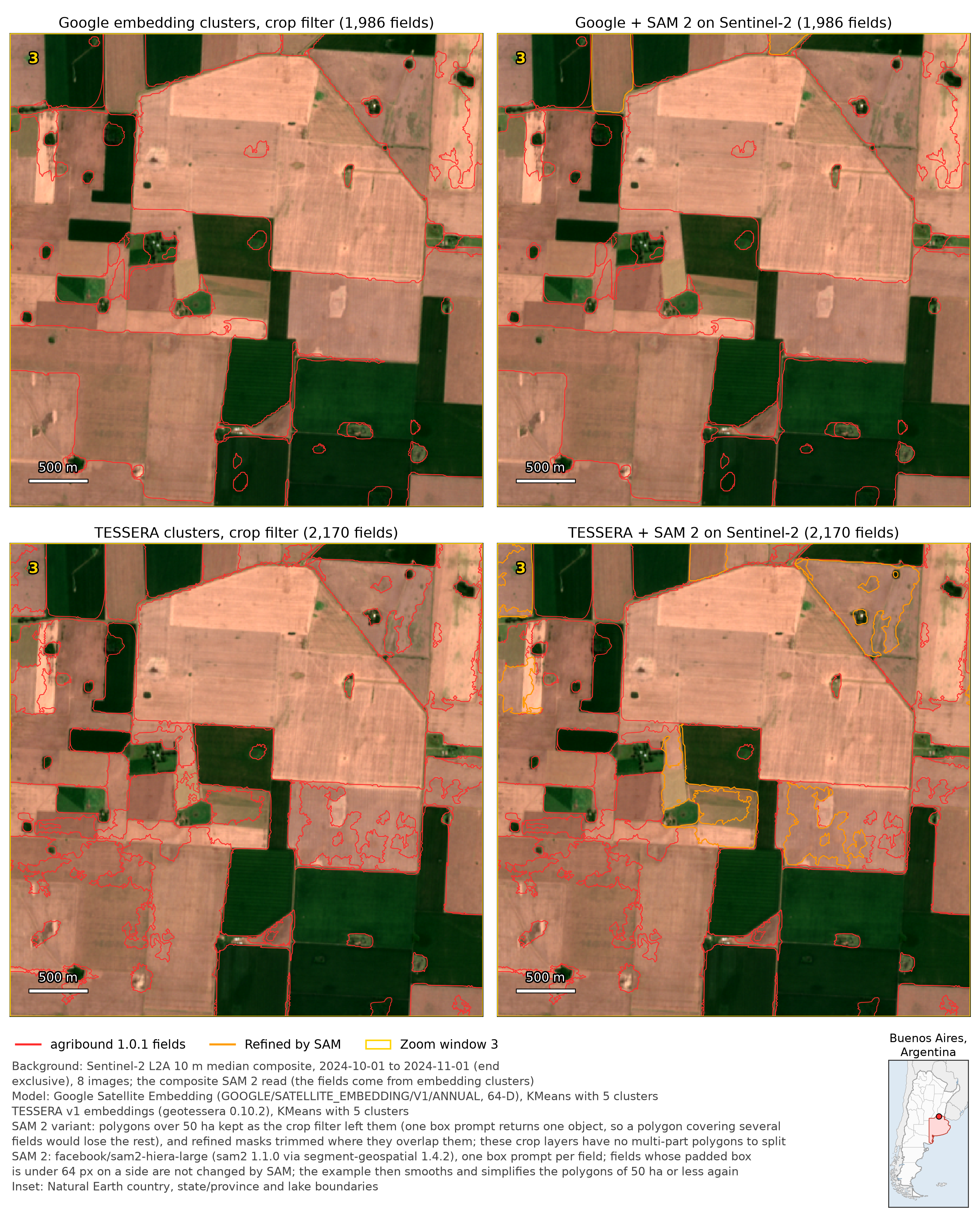
- Top: Google Satellite Embedding and TESSERA v1 clusters of 2024, after the crop filter and SAM 2 on a Sentinel-2 composite of October 2024, with parts over 50 ha kept unrefined (1,986 and 2,170 fields; see the next entry).
- Bottom left: Delineate Anything v2 on the same October 2024 Sentinel-2 composite (8 images): 2,818 fields (the crop filter kept 2,818 of 3,297).
- Bottom right: Delineate Anything v2 on SPOT 6/7 (6 m), 2023 (6 images; AIRBUS/SPOT6_7 ends on 2023-11-15): 3,306 fields (kept 3,306 of 3,761).
The two Delineate-Anything layers are the 1.0.0 outputs, which the 1.0.1 run reused. On Sentinel-2, Delineate-Anything outlines most pivots in the window as fields of their own and splits a few along tone changes inside the circle. On SPOT it leaves at least one faint pivot inside a larger rectangular field and breaks the two-tone pivot at the top left into pieces. The two inputs differ in date, season and resolution (SPOT: a 2023 median of 6 images at 6 m; Sentinel-2: an October 2024 median of 8 images at 10 m) and in crop-filter year (2023 and 2024); which of these differences causes the different outlines was not tested. Before SAM 2, 8 of the 14 pivots in the window have a TESSERA polygon of their own (IoU ≥ 0.8) and 7 a Google one (3 with 1.0.0); the others have a rougher polygon (IoU 0.5–0.8), are part of larger polygons or, for one Google pivot, have almost no polygon (see zoom 1 in the next entry). SAM 2 neither joins pieces nor splits merged polygons (it returns one polygon per input polygon). The pivots here are 40.5–56.8 ha, close to 50 ha, so some are refined (orange) and others keep their cluster outline (red). There is no reference layer here; the panels compare outlines, not accuracy.
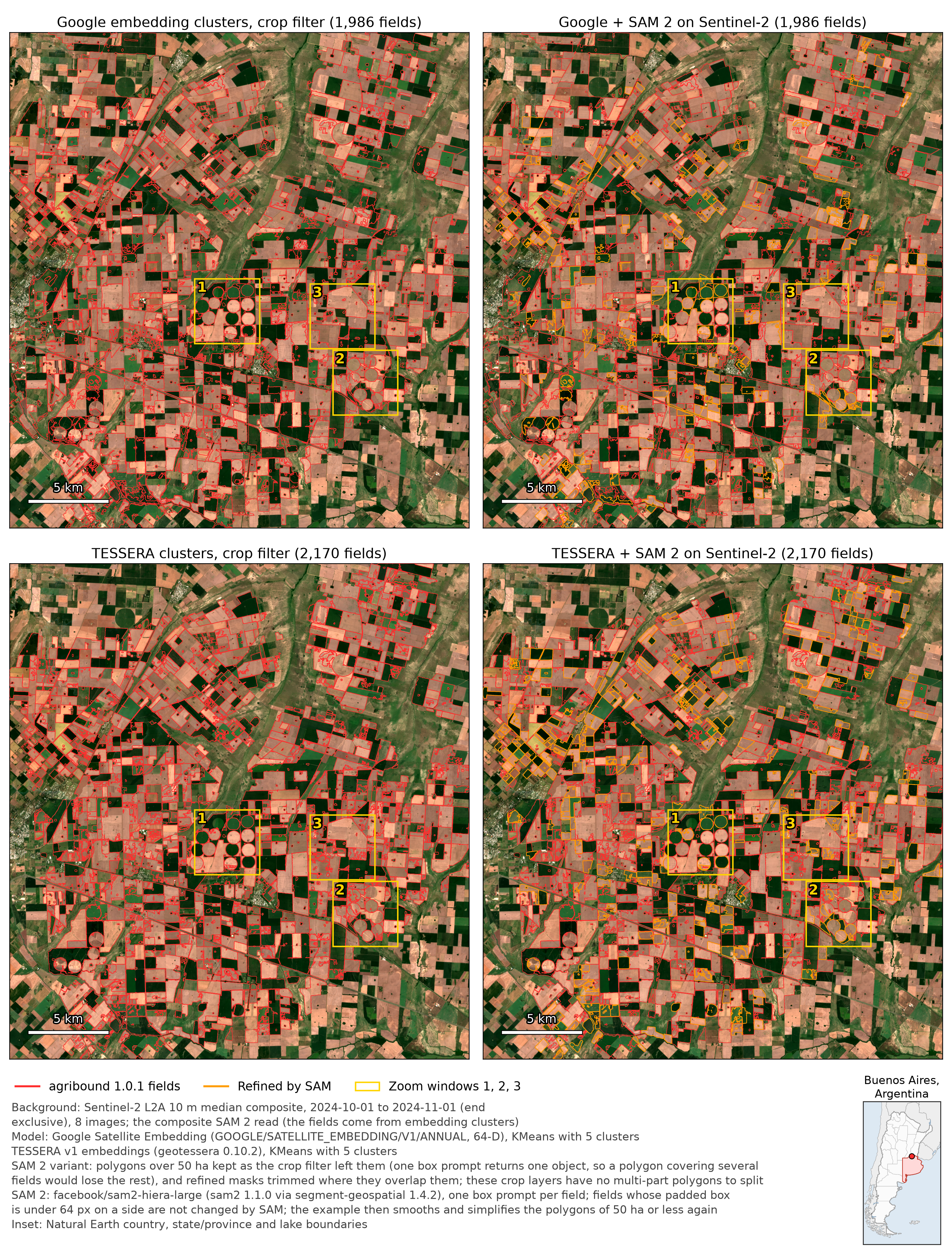
Pampas, Argentina — Google Satellite Embedding and TESSERA, whole study area and three zooms
Example 15 (steps 1–4) · Label-free: no training and no reference data · Pergamino partido, Buenos Aires Province, east of the city · min. area 5,000 m²; Dynamic World 2024 crop filter · the whole study area (a pentagon with a bounding box of about 28 × 31 km), then three 4 km windows (yellow squares 1–3).
Google Satellite Embedding (top) and TESSERA v1 (bottom) embeddings of 2024 are clustered (k = 5) and kept where they pass the crop filter (left): it kept 1,986 of 2,307 Google and 2,170 of 2,314 TESSERA polygons. SAM 2 then refines them on a Sentinel-2 composite of October 2024, 8 images (right), in the example's split variant: parts over 50 ha are kept unrefined (205 Google and 283 TESSERA polygons; neither crop layer has multi-part polygons, so nothing was split). Of the other 1,781 and 1,887 polygons, SAM 2 was prompted for 236 and 302 and refined 208 and 289. The other 28 and 13 masks covered less than half of their input polygon, so those polygons keep their input geometry; 1,545 and 1,585 polygons were below the size rule and were not prompted. SAM's overlap trim sees only the polygons it is given, so the example then trims the refined masks where they overlap the kept polygons (167 Google and 191 TESSERA masks). The 5,000 m² filter that follows removed no polygon: 1,986 and 2,170 remain, 208 and 289 of them refined (orange). The script smooths and simplifies the polygons of 50 ha or less again after SAM; the larger ones keep their crop-filter outline.
Each crop layer leaves a large group of fields without a polygon. In the TESSERA cluster raster, one cluster forms a connected region of 21,452 ha. Its representative point lies outside the study area, so the study-area rule drops it. In the Google cluster raster, a connected region of 11,105 ha is kept as one polygon, which the crop filter then removes. Delineate-Anything outlines 2,939 ha (TESSERA region) and 1,896 ha (Google region) of fields on Sentinel-2 in these regions; 2,893 ha and 1,881 ha of them are covered by no crop-filter polygon of that embedding (see Engines).
Why the split: SAM returns one object for each box prompt, and the refined
polygon replaces the whole input polygon when its mask covers at least
sam_min_coverage = 0.5 of it (the 1.0.1 default; 1.0.0 replaced it in every
case). Refining every polygon (fields_*_crop_sam2-s2_2024.gpkg) removed
4.9 % of the Google and 6.6 % of the TESSERA crop-filter area (EPSG:6933
sums); in that run, 70 Google and 37 TESSERA masks covered less than half of
their polygon and were not used. Of 29 centre pivots located in the composite
and checked by eye, 4 (Google) and 2 (TESSERA) were then less than half
covered by any polygon. Three of the Google ones had been part of a cluster
polygon more than twice their area (2.4 to 7.1 times); the fourth lay inside
the 11,105 ha polygon that the crop filter removed, so it had almost no
polygon already before SAM (0.4 % covered). Of the two TESSERA pivots, one
(2.4 % covered) had been part of a polygon 2.7 times its area and the other
(45.7 % covered) of one 1.8 times its area. With 1.0.0,
refining every polygon had removed 24 % and 16 % of the area and left 14 and
8 pivots less than half covered. With the split, 1 Google pivot and no
TESSERA pivot is less than half covered: the Google one is that pivot inside
the removed 11,105 ha polygon (0.2 % covered; see
SAM Refinement).
The split layers cover 0.8 % (Google) and 0.1 % (TESSERA) less ground than the
crop-filter polygons. They keep multi-field polygons as the clustering drew
them: 6 of the 29 pivots are inside a polygon more than twice their area in
the TESSERA layer, 9 in the Google layer, all of these polygons unrefined.
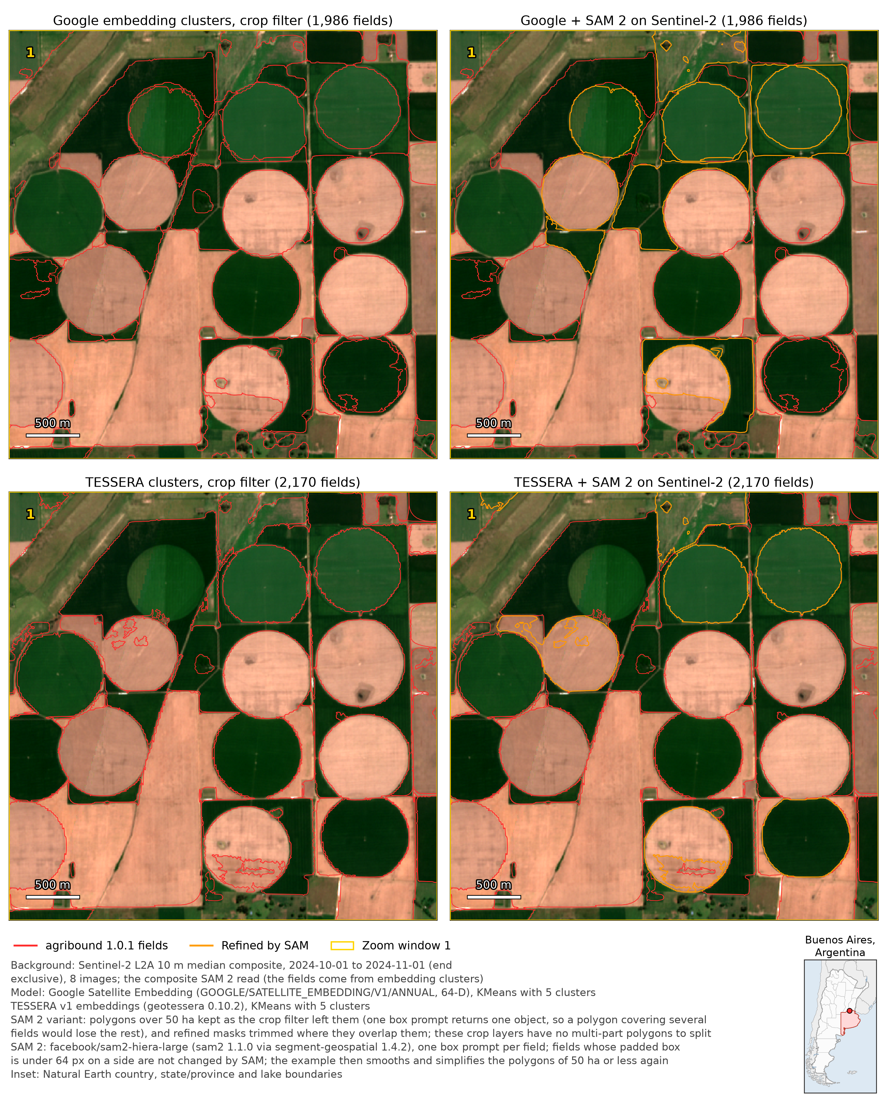
Zoom 1: centre pivots
The 4 km square with the most centre pivots (14 of the 29). The TESSERA clusters give 8 of them a polygon of their own (IoU ≥ 0.8) and 2 a rougher one (IoU 0.5–0.8). The other four, among them the two-tone pivot at the top left, are part of one 568.6 ha polygon, 10 to 14 times the area of each, which stays unrefined. The Google clusters give 7 pivots a polygon of their own and 2 a rougher one. Three at the left are part of one 137.2 ha polygon (2.4 to 2.6 times the area of each), and one at the bottom right shares an 89.3 ha polygon with the pivot above it (IoU 0.39). The dark-green pivot at the left edge has almost no Google polygon (0.4 % covered): it lay inside the 11,105 ha cluster polygon that the crop filter removed. With 1.0.0, the Google clusters gave only 3 of the 14 a polygon of their own and split several into pieces. SAM 2 redraws the outlines of the pivots it refines (orange) along their edges and can leave holes along within-field variation. With 1.0.1, refining every polygon leaves the four TESSERA pivots of the 568.6 ha polygon 94–98 % covered, because that polygon keeps its input geometry. With 1.0.0, refining every polygon had left them at most 7.4 % covered.
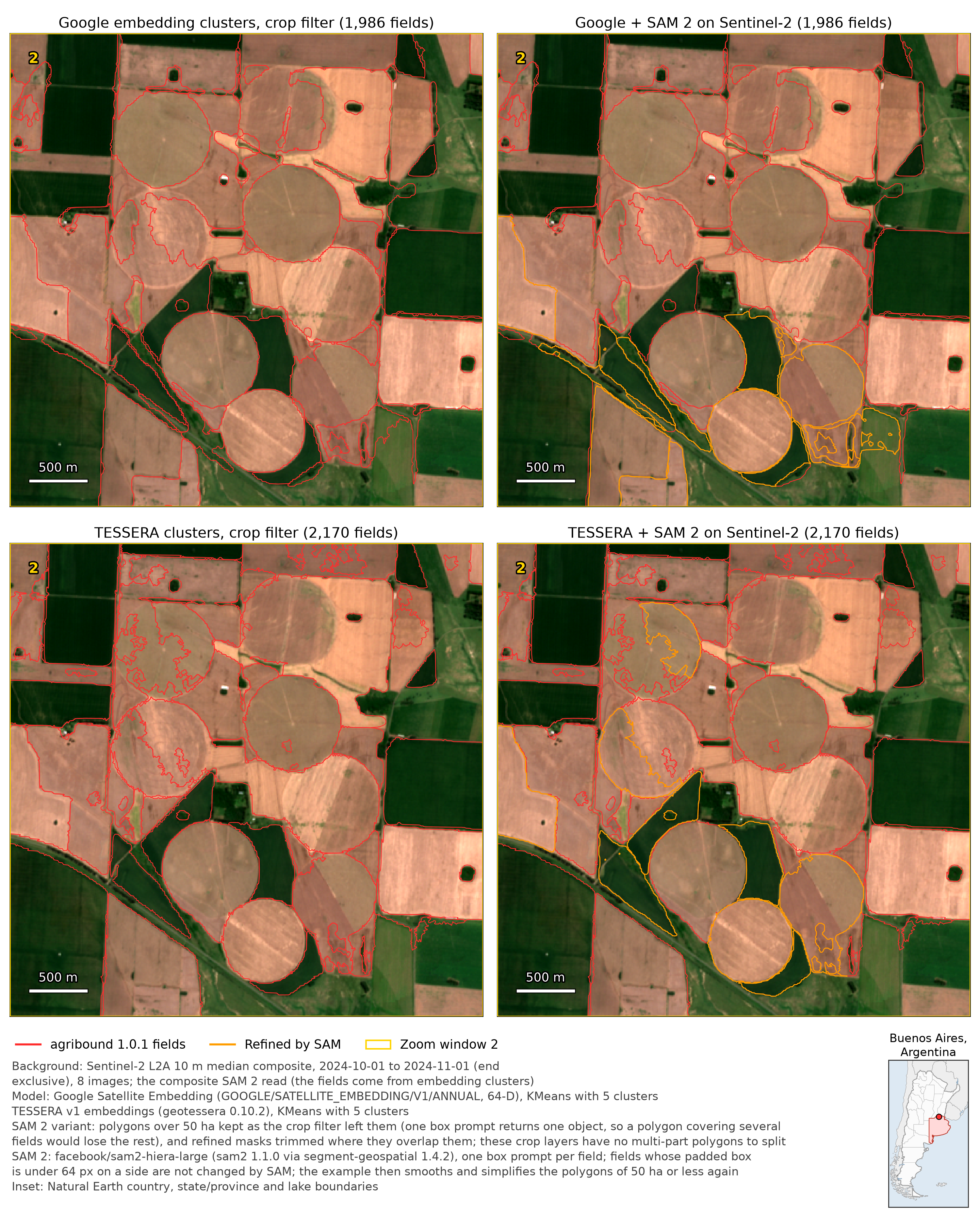
Zoom 2: centre pivots, south-east
A 4 km square around the south-east pivot group (8 of the 29 pivots), most of them bare in October 2024. One of them is part of a TESSERA polygon more than twice its area (114.1 ha, 2.2 times) and two are part of such Google polygons (2,639.3 ha, 45 times, and 125.0 ha, 2.4 times). Three more TESSERA pivots are in polygons of 104.6 ha (two pivots share it) and 110.0 ha, 1.8 to 1.9 times their area, and one more Google pivot is in a 94.4 ha polygon, 1.7 times its area. All of these polygons are over 50 ha and stay unrefined. Refining every polygon left 1 TESSERA pivot (45.7 % covered) and 1 Google pivot (5.6 %) of the 8 less than half covered. With 1.0.0, 5 TESSERA and 6 Google pivots here were part of polygons more than twice their area (the Google ones of a single 2,522 ha polygon), and refining every polygon had left 3 and 6 less than half covered.
Zoom 3: large merged polygons
This 4 km square (inside the study area, clear of zooms 1 and 2, with no checked pivot) is the one with the largest combined TESSERA and Google share of its area in crop-filter polygons over 200 ha, chosen on the 1.0.1 layers on 2026-09-29. 53.1 % of it is in four TESSERA polygons of 246.1 to 414.3 ha, each holding 6 to 12 Delineate-Anything Sentinel-2 fields of 5 ha or more (counting fields with at least 80 % of their area inside it), and 77.4 % in three Google polygons over 200 ha. The largest Google one, 2,639.3 ha, holds 92 such fields and also reaches into zoom 2. Both embeddings draw one outline around blocks of bare paddocks whose boundaries show in the composite. These polygons are over 50 ha, so the split variant leaves them unrefined. How many such merges the TESSERA clusters make depends on the k-means solution: the whole 1.0.1 TESSERA crop layer has 1 polygon over 500 ha (568.6 ha, in zoom 1), against 10 in 1.0.0 (see Engines). The 1.0.0 gallery used another window (centre 734400, 6249600), chosen by the share in polygons over 500 ha; on the 1.0.1 layers no TESSERA polygon over 500 ha touches it.
Compared with the 0.1.x README image
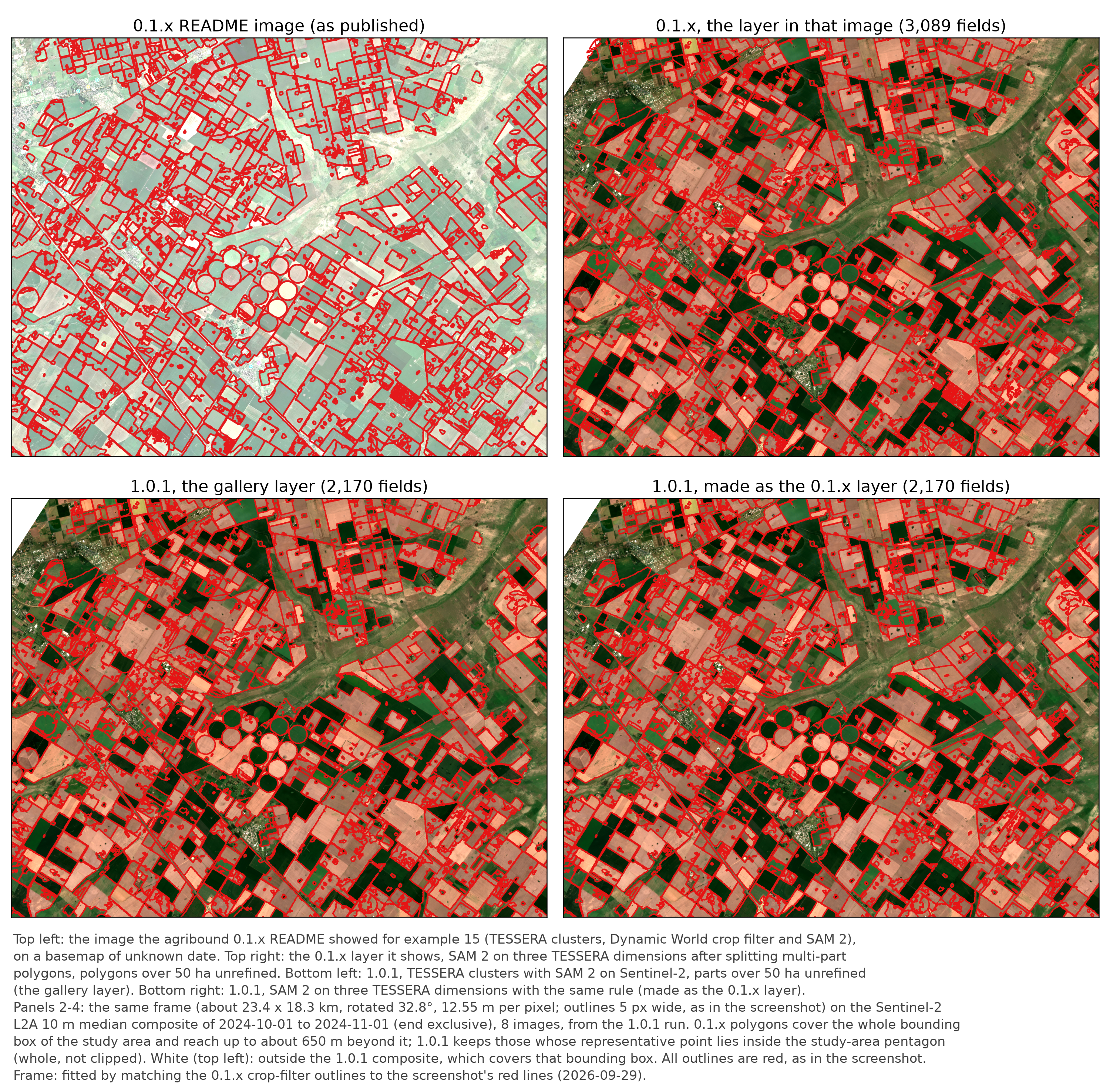
The agribound 0.1.x README showed this example as a wide screenshot (top
left): about 23 × 18 km, rotated, with outlines about 63 m wide, of the 0.1.x
layer with SAM 2 on three TESSERA dimensions and polygons over 50 ha
unrefined (its caption said SAM 2 on Sentinel-2). Drawn in the same frame with
the same line width, the 0.1.x layer (top right) and the two 1.0.1 split layers
(bottom: the gallery layer, and SAM 2 on three TESSERA dimensions as in 0.1.x)
look much alike: at this scale single pixels, small fragments and merged
fields are hard to see, which is why the 4 km zooms above look rougher than
the 0.1.x image. By their polygon sizes, the 1.0.1 TESSERA clusters are closer
to the 0.1.x ones than the 1.0.0 clusters were. In the crop-filter layers,
15.5 % (0.1.x), 38.4 % (1.0.0) and 18.2 % (1.0.1) of the area is in polygons
over 200 ha, and the largest polygon is 566, 1,447 and 568 ha (EPSG:6933);
7, 10 and 6 of the 29 pivots are part of a polygon more than twice their area.
The cluster labels were not compared pixel by pixel (see
Engines). The 1.0.1
clusters sit about a pixel further east than the 0.1.x ones (1.0.1 reused the
TESSERA raster that 1.0.0 built; see
Satellite Sources). Unlike the
other images, it has no inset, and its footer names the imagery but not the
models; the 1.0.1 layers use the models and versions of the entries above. The
image is rendered by tools/make_gallery_pampas_0.1x.py.
India, West Bengal — FTW on Sentinel-2 vs Delineate-Anything on SPOT-Pan
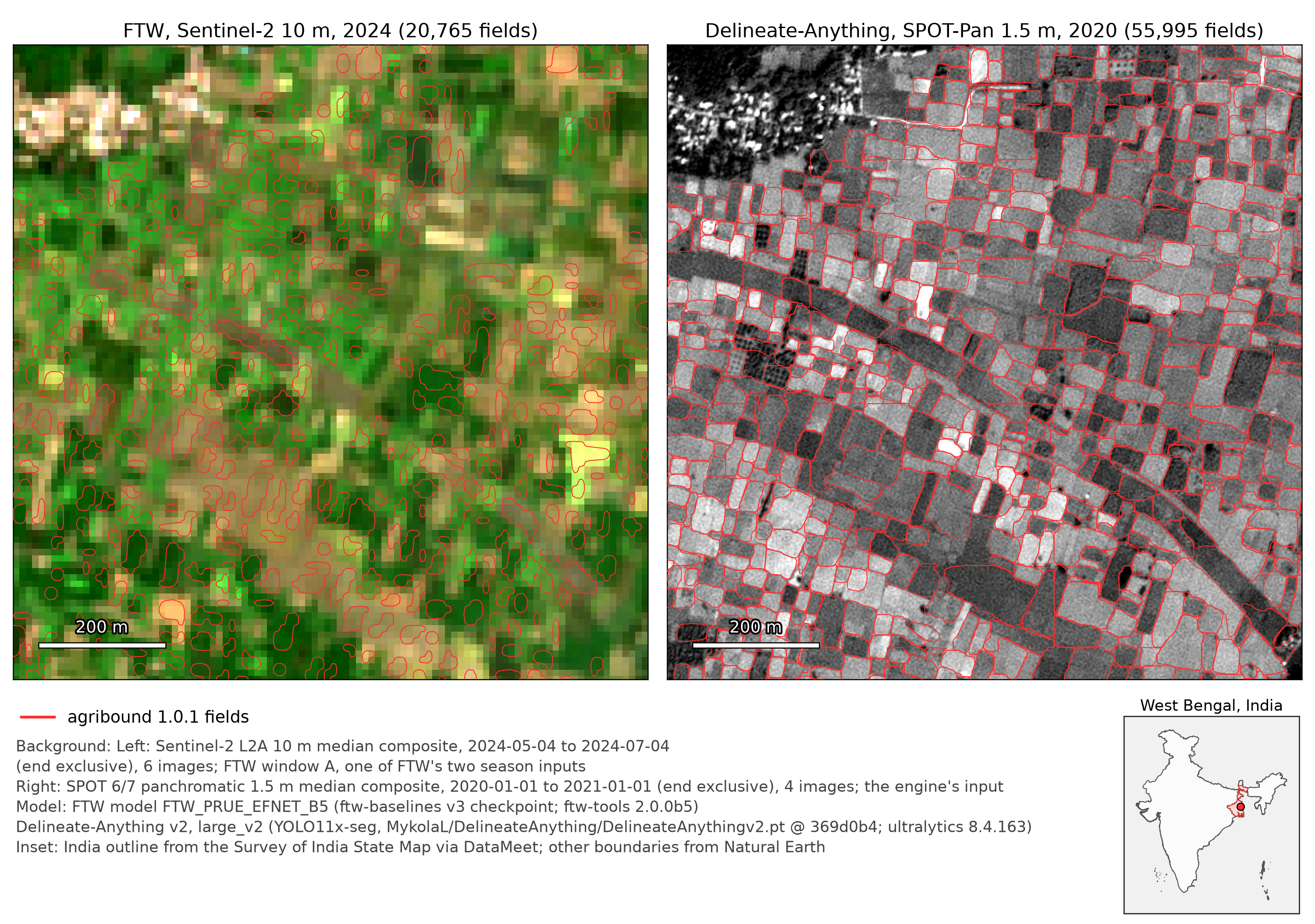
Example 02 · Label-free · Nadia District, West Bengal, between Nabadwip and Krishnanagar (study area 88.35–88.50° E, 23.35–23.50° N; about 95 % in Nadia, the north-western corner west of the Bhagirathi in Purba Bardhaman) · min. area 100 m² · the same 1 km window in both panels (in Krishnagar-I block, centre 23.39° N, 88.42° E; the square with the most Delineate-Anything polygons), four years apart.
- Left: FTW on Sentinel-2 2024, with two season windows, 4 May–3 Jul 2024 (6 images, shown) and 25 Nov 2024–24 Jan 2025 (18 images); Dynamic World 2024 crop filter. The window is about 100 × 100 Sentinel-2 pixels.
- Right: Delineate Anything v2 on SPOT 6/7 panchromatic (1.5 m), 2020 (4 images; restricted SPOT access); Dynamic World 2020 crop filter.
FTW produced 63,485 polygons. Of these, 62,110 fall inside the study area (the composite covers its bounding box), 49,800 pass the 100 m² filter, and the crop filter kept 20,765 of those 49,800. Their median area is 0.04 ha, about four Sentinel-2 pixels. In this window they do not follow the field edges visible in the SPOT-Pan image. Delineate Anything v2 produced 80,045 polygons (78,340 inside the study area, 78,083 after the 100 m² filter); the crop filter kept 55,995 of 78,083, with a median area of 0.12 ha. Both layers are the 1.0.0 outputs, which the 1.0.1 run reused. There is no reference data here; neither output was evaluated. The example also clusters Google Satellite Embedding and TESSERA embeddings (not shown; Google with k = 5 chosen automatically, TESSERA with a fixed k = 8). With 1.0.1 the crop filter kept 1,465 of 9,628 Google and 11,722 of 79,712 TESSERA polygons (3,850.2 and 5,707.3 ha); with 1.0.0 it kept 1,230 and 8,818 (3,341.0 and 5,773.8 ha).
Global South — Delineate-Anything v2 on SPOT 6/7 panchromatic, six landscapes
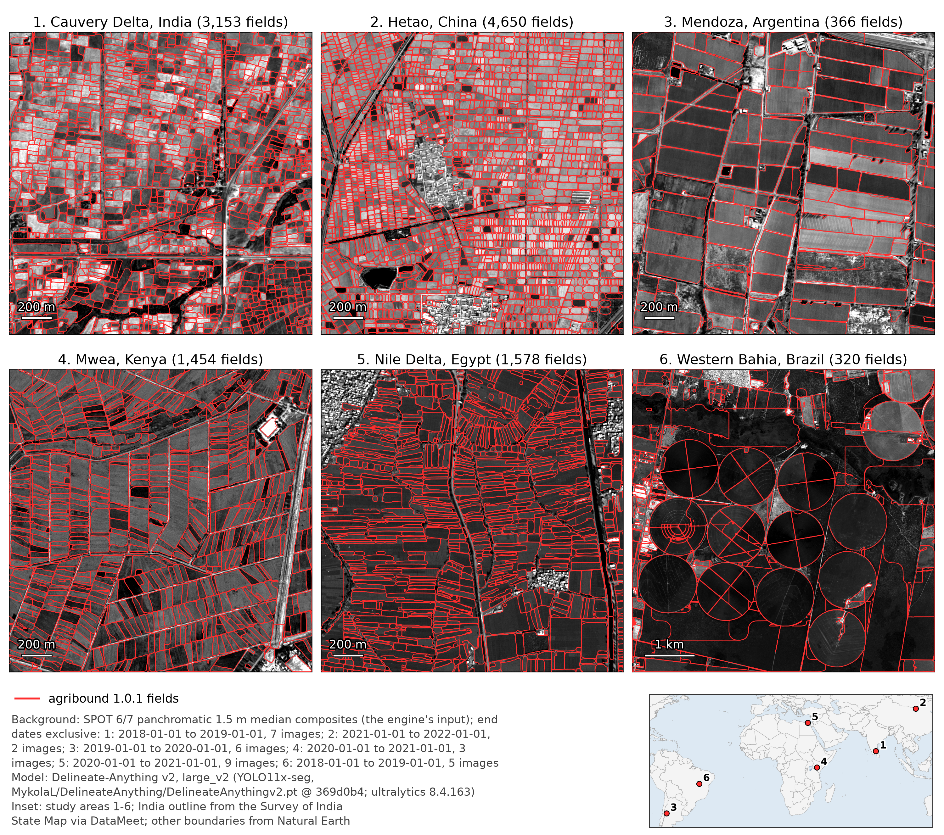
Example 22 · Label-free · six study areas, each a 3 km square in its UTM zone (6 km in western Bahia, where the pivots are about 1 km across) · min. area 100 m² · no crop filter on the maps (see below) · in each panel, the densest of the 2 km squares whose centres lie on a 1 km grid (four per 3 km area), at about 2 m per pixel of the full-size image; in western Bahia, the whole 6 km study area (about 6 m per pixel).
Delineate Anything v2 as released on SPOT 6/7 panchromatic 1.5 m composites (restricted SPOT access), the median of one calendar year's scenes with at most 15 % cloud cover. The years were chosen so that 2 to 6 scenes cover each square and none covers only part of it (image counts in the footer include selected scenes with no pixels in the square).
| # | Study area | Year | Fields | Median (ha) | Crop filter kept |
|---|---|---|---|---|---|
| 1 | Cauvery Delta, Tamil Nadu, India | 2018 | 3,153 | 0.18 | 3,001 |
| 2 | Hetao irrigation district, Inner Mongolia, China | 2021 | 4,650 | 0.11 | 3,826 |
| 3 | Agrelo, Mendoza, Argentina | 2019 | 366 | 1.24 | 344 |
| 4 | Mwea irrigation scheme, Kenya | 2020 | 1,454 | 0.39 | 1,361 |
| 5 | Nile Delta near Tanta, Egypt | 2020 | 1,578 | 0.19 | 1,460 |
| 6 | Luís Eduardo Magalhães, western Bahia, Brazil | 2018 | 320 | 1.14 | 47 |
The fields range from small paddies and strip plots to vineyard blocks and
centre pivots about 1 km across. The model follows the bunds of the Cauvery
Delta paddies and the Mwea tenant strips and outlines the Mendoza vineyard
blocks along their windbreaks. In Hetao it draws many polygons smaller than
the canal-grid blocks. In the Nile Delta it joins neighbouring strips: west of
the square shown, one polygon of about 105 ha covers a whole block of strip
plots between two drains. Of the 13 pivots wholly inside the Bahia panel it
splits eight (four into quarters, two into seven and eleven pieces along their
sector lines, one into rings and one into halves along an airstrip) and
outlines five whole; its two largest polygons there (161 and 151 ha) are
blocks between the pivots. There is no reference data here, so these are
outlines, not accuracy. The crop filter (Dynamic World of each year, mean
crops probability at least 0.3) runs as a separate step in the example. It
kept 47 of the 320 Bahia polygons: over the other 273 the mean Dynamic World
crops probability is below 0.3. The maps therefore show the unfiltered
polygons. The inset is a world map with the six study areas numbered as the
panels.
Tree crops — Delineate-Anything v2 on SPOT 6/7 panchromatic, four landscapes
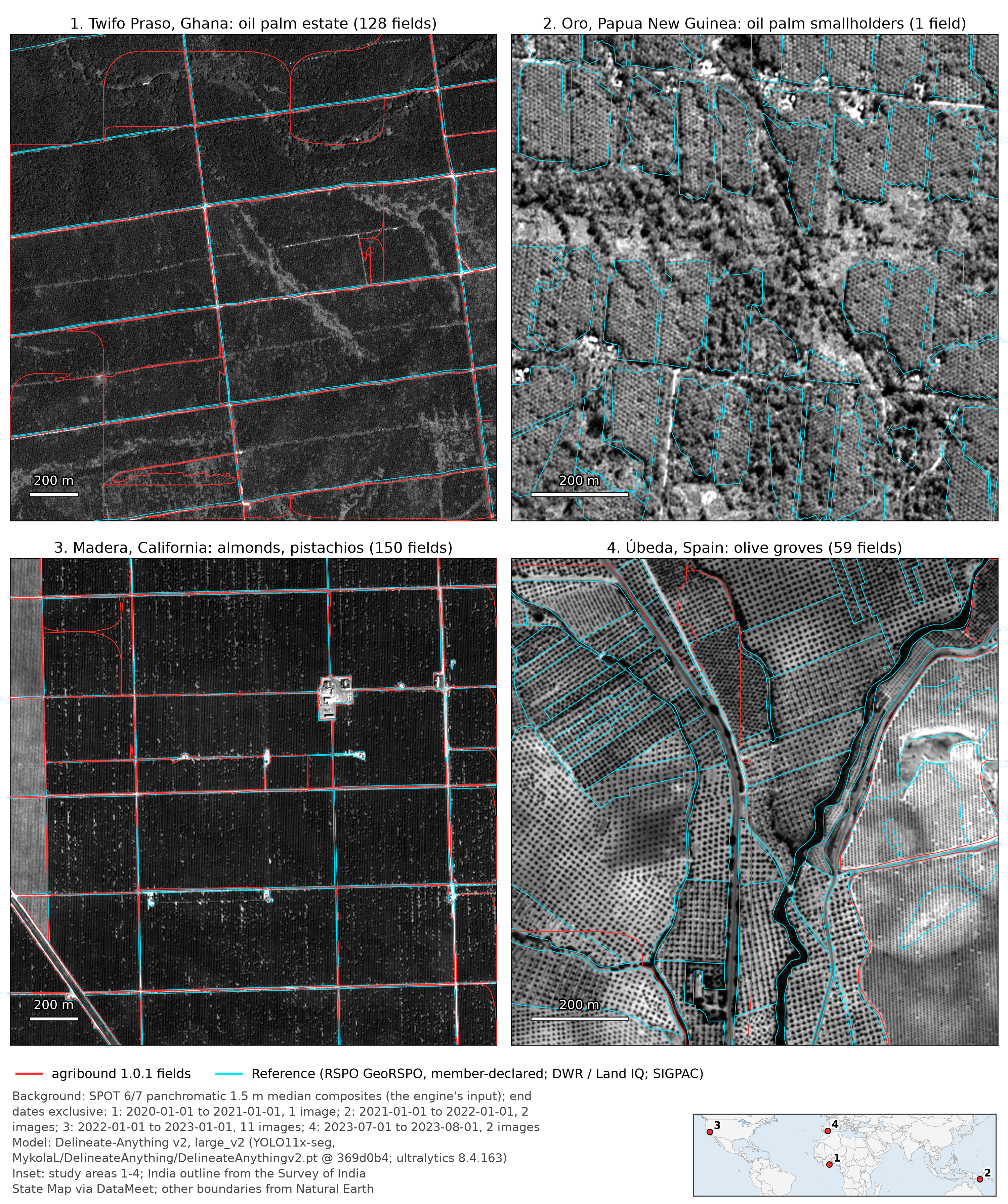
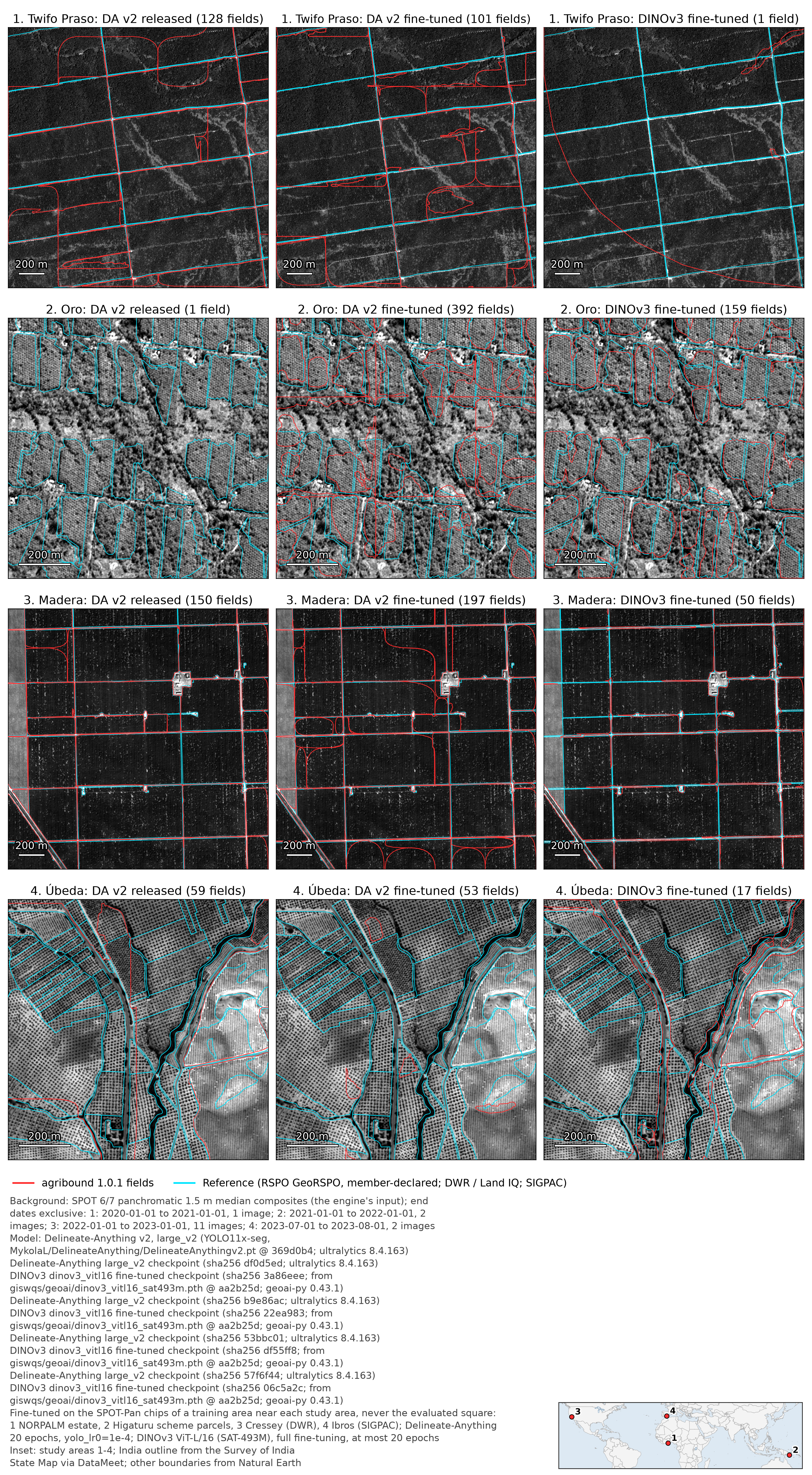
Example 23 · Released weights (no fine-tuning) · four study areas, squares of 3 to 5 km in their UTM zones · min. area 2,500 m² · no crop filter on the maps (see below) · in each panel, the square with the most reference polygons (2 km at Twifo Praso and Madera, 1 km at Oro and Úbeda).
Delineate Anything v2 as released on SPOT 6/7 panchromatic 1.5 m composites (restricted SPOT access) of one year per study area, with the reference polygons in cyan: the RSPO GeoRSPO concession maps (member-declared, published in September 2026) for an industrial oil palm estate and for oil palm smallholders, the DWR / Land IQ crop map of water year 2022 for almond and pistachio orchards, and SIGPAC parcels ("recintos") of the 2025 campaign for olive groves. Fields match at IoU ≥ 0.5. Precision counts only the predictions that overlap a reference polygon, because the RSPO maps of Twifo Praso and Oro do not map every field in their squares; in Madera and Úbeda, whose references map all fields, the scores are those of the tree-crop fields.
Only at Twifo Praso and Oro has the model seen none of the fields. Delineate Anything v2 was trained on FBIS-73M, which has no patches in Ghana or Papua New Guinea, but whose training patches cover the Madera square, with field labels that match the DWR / Land IQ polygons (121 of the 122 reference fields appear as training labels at IoU ≥ 0.5), and 87 % of the Úbeda square, with labels that follow SIGPAC (166 of the 225 recintos). This was checked against the public FBIS-73M patch list, images and labels (patch footprints and label polygons); the dataset does not name its sources.
| # | Study area | Year | Reference (tree crops) | Fields | Recall | Precision | F1 | Crop filter kept: default / tree crops |
|---|---|---|---|---|---|---|---|---|
| 1 | Twifo Praso, Ghana: oil palm estate | 2020 | 55 blocks, median 39.9 ha | 128 | 0.45 | 0.21 | 0.29 | 0 / 128 |
| 2 | Oro Province, Papua New Guinea: oil palm smallholders | 2021 | 302 parcels, median 1.5 ha | 1 | 0.003 | 1 of 1 | 0.007 | 0 / 1 |
| 3 | Madera County, California: almonds and pistachios | 2022 | 112 of 122 fields, median 16.6 ha | 150 | 0.83 | 0.89 | 0.86 | 149 / 149 |
| 4 | Úbeda, Jaén, Spain: olive groves | 2023 | 212 of 225 recintos, median 3.2 ha | 59 | 0.04 | 0.19 | 0.07 | 18 / 26 |
Where the trees grow in blocks separated by roads, the released model finds the blocks: 83 % of the Madera orchards, and 45 % of the Twifo estate blocks. At Twifo it also splits about half of the blocks (split rate 0.49), so most of its other polygons lie on reference blocks. Many blocks are cut along the straight north-south and east-west edges of the engine's 768 m inference tiles (every 384 m): 54 of the 55 blocks are longer than a tile, and the engine does not join pieces of a field that meet at a tile edge without overlapping. About as many split blocks are cut along a road or track that runs through the block, and some along lines that follow nothing in the image. Where the parcels are stands of trees among other trees, it finds almost nothing: one polygon at Oro, where the parcels show the planting grid of the palms. At Úbeda the recintos follow cadastral lines that cross uniform groves; after dropping recintos under 2,500 m² and joining touching recintos of the same land use (46 tree-crop groves of 57) recall is 0.20 and precision 0.26.
The crop filter runs as a separate step in the example, twice. The default
rule (Dynamic World outside the conterminous US, NLCD inside) removes every
polygon of panels 1 and 2 (Twifo Praso and Oro): it also removes all 55 Twifo
and all 302 Oro reference polygons, and keeps 46 of the 225 Úbeda recintos.
lulc_tree_crops=True (Dynamic World crops + trees) keeps all these
polygons and all the Twifo and Oro reference polygons, and 108 of the Úbeda
recintos. In Madera the filter uses
NLCD, whose cultivated-crops class includes orchards, and keeps all 122
reference fields with either rule. The maps therefore show the unfiltered
polygons. The inset is a world map with the four study areas numbered as the
panels.
Thanks to Jacob Abramowitz (The University of Alabama in Huntsville), who asked about tree crops and pointed to the RSPO concession maps. The RSPO polygons are member-declared, are provided "for informational and illustrative communication purposes only" (RSPO Disclaimer for Map Publication) and are not redistributed here; the example downloads them from RSPO.
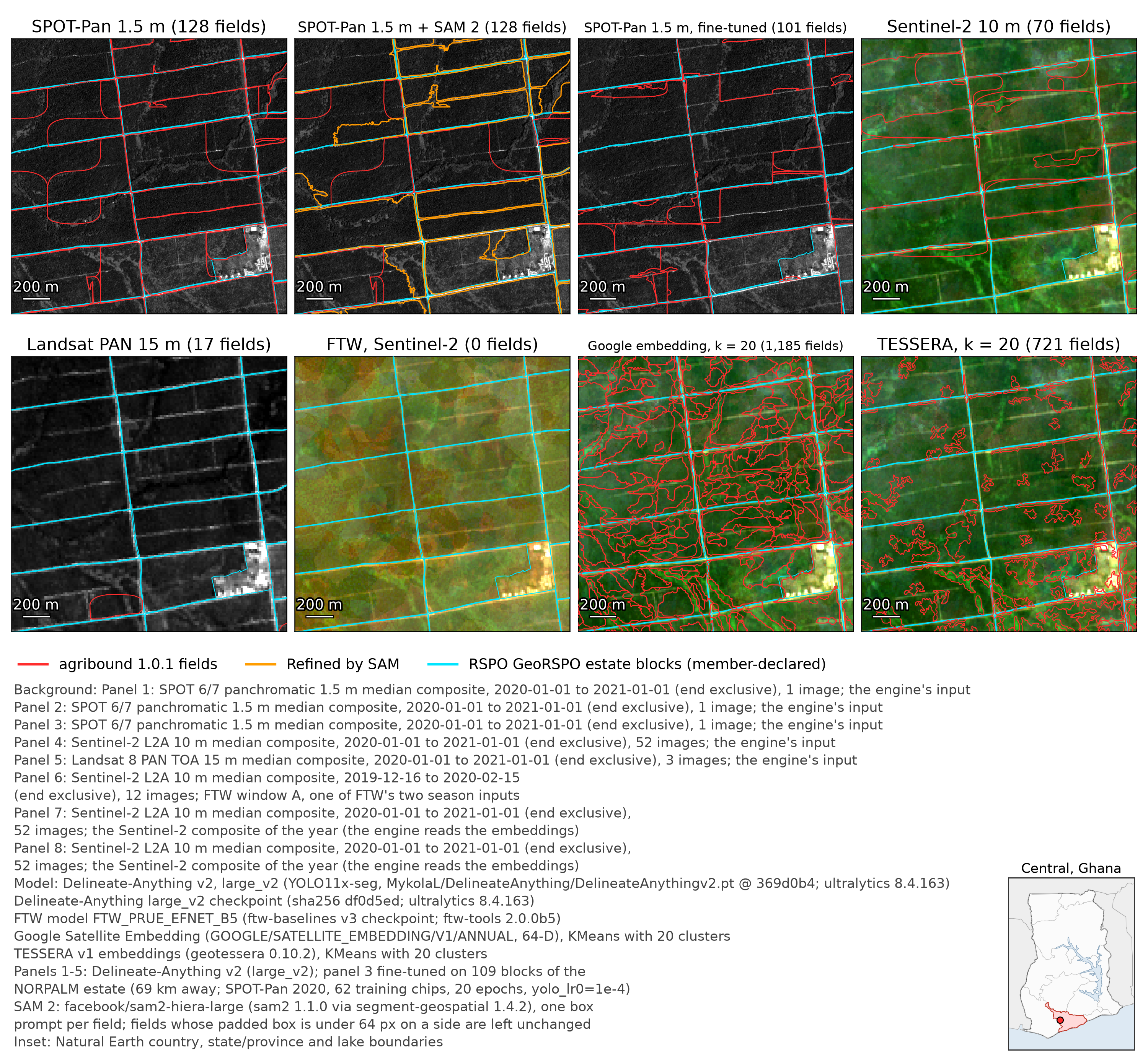
Twifo Praso, Ghana — oil palm estate blocks from SPOT-Pan 1.5 m to Landsat PAN 15 m
Example 23 · Reference: the estate's RSPO GeoRSPO blocks (55 with their representative point in the 5 km square, median 39.9 ha) · 2020 for every source · min. area 2,500 m² · no crop filter on the maps · the 2 km square with the most reference blocks.
| Panel | Fields | Recall | Precision | F1 | Mean IoU | Boundary F1 (10 m) | Merged | Split |
|---|---|---|---|---|---|---|---|---|
| Delineate-Anything v2, SPOT-Pan | 128 | 0.45 | 0.21 | 0.29 | 0.75 | 0.56 | 0.04 | 0.49 |
| + SAM 2 | 128 | 0.40 | 0.20 | 0.27 | 0.78 | 0.46 | 0.02 | 0.45 |
| Fine-tuned (NORPALM), SPOT-Pan | 101 | 0.31 | 0.18 | 0.23 | 0.72 | 0.46 | 0.60 | 0.45 |
| Delineate-Anything v2, Sentinel-2 | 70 | 0.27 | 0.22 | 0.24 | 0.73 | 0.41 | 0.15 | 0.25 |
| Delineate-Anything v2, Landsat PAN | 17 | 0.05 | 0.18 | 0.08 | 0.88 | 0.15 | 0.02 | 0.05 |
| FTW, Sentinel-2 | 0 | 0 | - | 0 | - | 0 | - | - |
| Google embedding, k = 20 | 1,185 | 0 | 0 | 0 | - | 0.17 | 0.07 | 0.76 |
| TESSERA, k = 20 | 721 | 0 | 0 | 0 | - | 0.17 | 0.02 | 0.11 |
Precision counts the predictions that overlap a reference block (the square
also holds a village and forest outside the estate). A block is merged when
the prediction covering most of it also covers a quarter of another block,
and split when two predictions each cover a tenth of it. The blocks are
separated by gaps of about 4 m along the roads, sharp on SPOT-Pan and less
than a pixel wide on Sentinel-2 and Landsat PAN. On SPOT-Pan the released
model follows the roads, but about half of the blocks come out in pieces
(split rate 0.49). Many are cut along the straight edges of the 768 m
inference tiles (every 384 m), because a block of about 1 km is longer than a
tile and the engine does not join pieces that meet at a tile edge without
overlapping. About as many are cut along a road or track that runs through
the block, which the model follows too, and some along lines that follow
nothing in the image. SAM 2 refined 102 of the 128 polygons; it raised the mean
IoU of the matched blocks and lowered recall. The fine-tuned model was trained
on the blocks of the NORPALM estate, 69 km from the Twifo square (centres 81 km
apart), on SPOT-Pan of the same year (62 training chips, 20 epochs,
yolo_lr0=1e-4; validation mask mAP50 0.47, where the released weights scored
0.17 on the same chips in a separate test); on Twifo it merges 60 % of the
blocks with a neighbour and finds fewer blocks than the released model. The
Landsat 8 PAN composite (3 images) shows the road grid, but the model draws
only 17 polygons. FTW predicted no field pixels from its two Sentinel-2 windows
(2019-12-16 to 2020-02-14 and 2020-07-16 to 2020-09-14, 12 and 7 images, set to
clear months because oil palm has no crop season), and the embedding clusters
are land-cover segments that match no block. Against the estate outline (the
blocks joined), the 128 SPOT-Pan polygons of the released model cover 73 % of
the estate's area in the square and put 3.5 % of their area (61 ha) outside it;
the 121 with their representative point in the estate put 0.2 % of their area
outside it. The default crop filter removes every polygon of every panel;
lulc_tree_crops=True keeps all but three Google and four TESSERA segments.
The embedding panels are drawn on the Sentinel-2 composite of the same year.
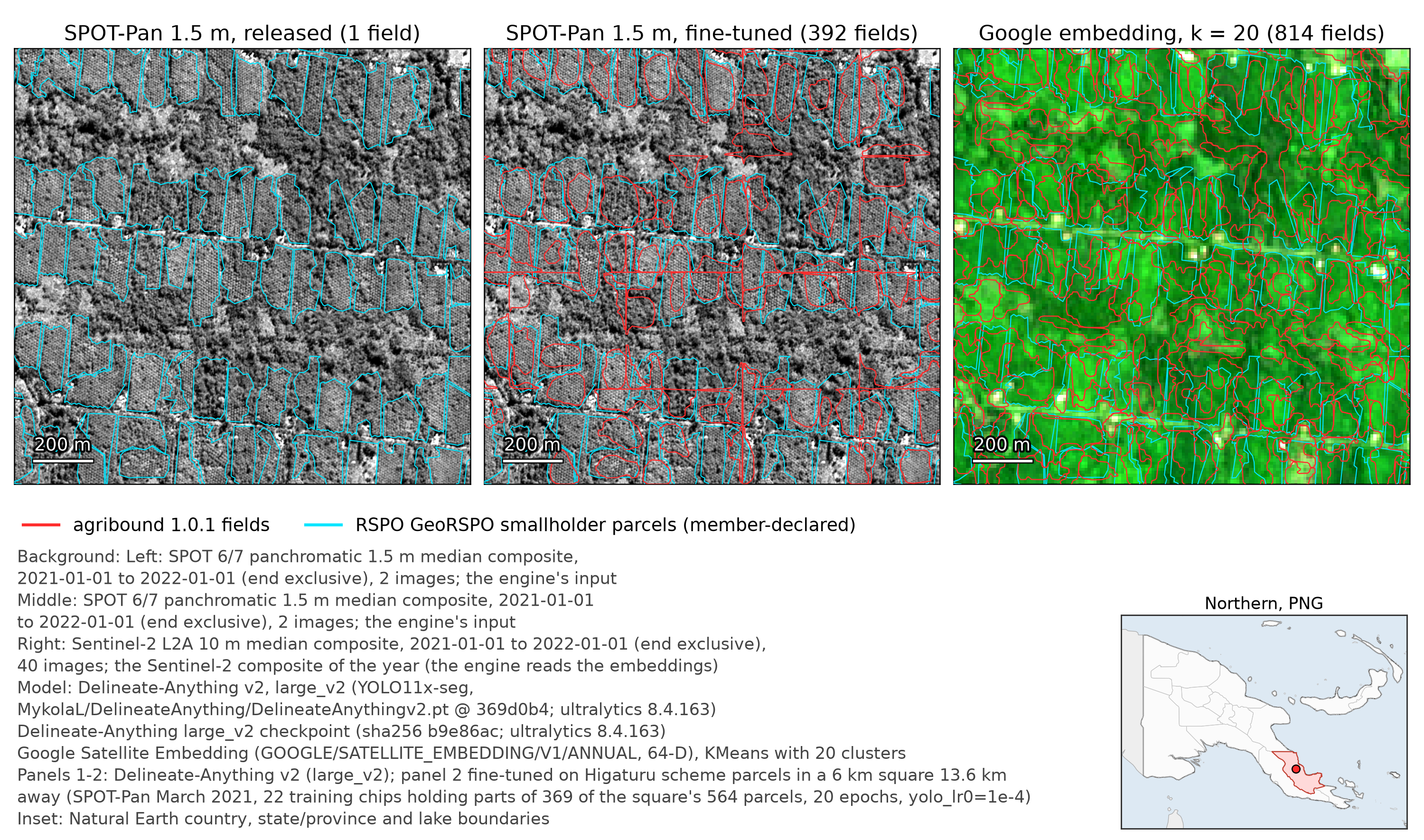
Oro Province, Papua New Guinea — oil palm smallholder parcels, released and fine-tuned models
Example 23 · Reference: RSPO GeoRSPO parcels of the Higaturu scheme (302 with their representative point in the 3 km square, median 1.5 ha; they cover about half of it) · 2021 · min. area 2,500 m² · no crop filter on the maps · the 1.5 km square with the most reference parcels.
The released Delineate Anything v2 made one detection on the SPOT-Pan
composite of the square (81 inference tiles), and none on Sentinel-2 or
Landsat PAN; FTW predicted no field pixels. Fine-tuned on parcels of the same
scheme in a 6 km square 13.6 km from the Oro square (centres 19.5 km apart;
SPOT-Pan of March 2021; 22 training chips with at least a quarter of their
pixels labelled, which hold parts of 369 of the 564 parcels in the square; 20
epochs, yolo_lr0=1e-4), it drew
392 polygons and matched 68 of the 302 parcels (recall 0.23; precision 0.19,
or 0.20 among the predictions with at least half of their area within 20 m of
a parcel; mean IoU of the matches 0.61; boundary F1 0.41 at 10 m). The long
straight north-south and east-west lines in the fine-tuned panel lie on edges
of the 768 m inference tiles (every 384 m): 22 % of its boundary length is
within 2 m of a tile edge, where 2 % would be by chance. The Google Satellite
Embedding clusters (814
segments) match 8 % of the parcels. Precision cannot count the palm stands
that the reference leaves out: about half of the square is not mapped. The
fine-tuned model was added to the example after the released model's result
here, and kept after its own Oro score was seen; none of its settings was
changed after that score, and its training parcels, digitised by the same
RSPO member, share no parcel with the Oro reference. Both
crop-filter rules were applied: the default one keeps none of the 302
reference parcels, lulc_tree_crops=True keeps all of them. The embedding
panel is drawn on the Sentinel-2 composite of the same year.
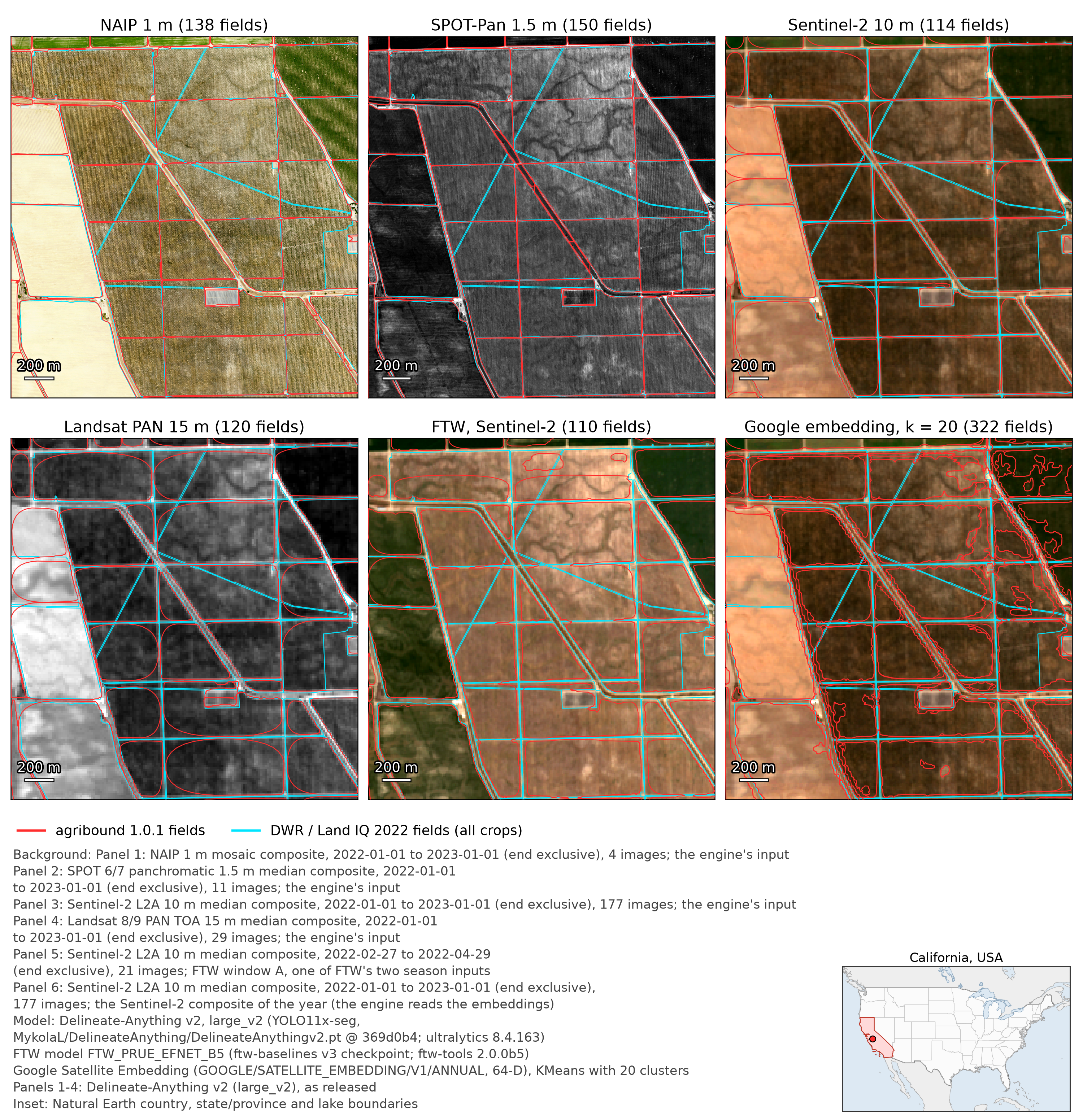
Madera County, California — almond and pistachio orchards from NAIP 1 m to Landsat PAN 15 m
Example 23 · Not unseen fields: Delineate Anything v2's training data (FBIS-73M) cover this square, with labels that match 121 of its 122 reference fields · Reference: the DWR / Land IQ crop map of water year 2022 (122 fields with their representative point in the 5 km square, 112 of them almond or pistachio orchards, median 16.6 ha) · 2022 for every source · scores of the orchards · min. area 2,500 m² · no crop filter on the maps (the default filter, NLCD here, removes at most 4 polygons of a layer) · the 2.5 km square with the most reference fields.
| Panel | Fields | Recall | Precision | F1 | Mean IoU | Boundary F1 (10 m) | Merged |
|---|---|---|---|---|---|---|---|
| Delineate-Anything v2, NAIP | 138 | 0.70 | 0.80 | 0.74 | 0.88 | 0.85 | 0.40 |
| Delineate-Anything v2, SPOT-Pan | 150 | 0.83 | 0.89 | 0.86 | 0.90 | 0.89 | 0.29 |
| Delineate-Anything v2, Sentinel-2 | 114 | 0.70 | 0.91 | 0.79 | 0.85 | 0.70 | 0.26 |
| Delineate-Anything v2, Landsat PAN | 120 | 0.71 | 0.87 | 0.78 | 0.81 | 0.51 | 0.31 |
| FTW, Sentinel-2 | 110 | 0.54 | 0.74 | 0.63 | 0.73 | 0.12 | 0.38 |
| Google embedding, k = 20 | 322 | 0.54 | 0.21 | 0.30 | 0.72 | 0.27 | 0.39 |
The orchards are blocks of 16.6 ha (median) separated by roads, and every approach shown finds most of them: Delineate Anything v2 at all four resolutions, even 15 m Landsat PAN, which is outside its 0.25-10 m training range (Landsat 8 and 9, 29 images), and FTW. SAM 2 on the SPOT-Pan polygons (not shown) changed little (F1 0.84), and TESSERA clusters (not shown) matched 48 of the 112 orchards (recall 0.43, F1 0.13). The reference splits some blocks along narrow tracks (the diagonal cyan lines) that no output draws, so a prediction over such a block covers parts of two reference fields (merge rates of 0.26 to 0.40 for Delineate-Anything). The embedding panel is drawn on the Sentinel-2 composite of the same year.
Tree crops — Delineate-Anything v2, released and fine-tuned, against DINOv3 fine-tuned
Example 23 · SPOT 6/7 panchromatic 1.5 m · fine-tuned models trained near each study area, never on the evaluated square · in each row, the square with the most reference polygons (2 km at Twifo Praso and Madera, 1 km at Oro and Úbeda), the same for the three models.
Delineate Anything v2 predicts each field as an object. DINOv3 (a ViT-L/16
backbone pre-trained on SAT-493M satellite imagery, with a DPT head) labels
each pixel as background, field interior or field boundary, and the fields
are its interior regions. It has no published field-boundary weights, so it
was fine-tuned only; Delineate Anything v2 is shown as released and
fine-tuned. Both were fine-tuned on the same labels and SPOT-Pan composite of
a training area: the NORPALM estate for Twifo Praso, Higaturu scheme parcels
for Oro, a 5 km square of DWR / Land IQ fields near Cressey, 41.9 km from the
Madera square (centres 48.3 km apart), and a 4 km square of SIGPAC recintos
around Ibros, 10.8 km from the Úbeda square (centres 16.1 km apart). The last
two squares were chosen by a fixed rule from the labels and the imagery before
any model was trained on them, and no model's settings were changed after it
was scored. The Delineate-Anything fine-tuning for Oro was added after the
released model's Oro result and kept after its own Oro score was seen (see the
Oro entry). Each model uses agribound's default recipe, except yolo_lr0=1e-4
for Delineate-Anything (the default is 0.002), set on the NORPALM validation
chips: Delineate-Anything with Ultralytics' augmentation, DINOv3 with full
fine-tuning, no augmentation and at most 20 epochs (early stopping on the
validation loss).
| Study area | Model | Fields | Recall | Precision | F1 | Mean IoU | Boundary F1 (10 m) | Merged | Split |
|---|---|---|---|---|---|---|---|---|---|
| 1 Twifo Praso | Delineate-Anything v2, released | 128 | 0.45 | 0.21 | 0.29 | 0.75 | 0.56 | 0.04 | 0.49 |
| Delineate-Anything v2, fine-tuned | 101 | 0.31 | 0.18 | 0.23 | 0.72 | 0.46 | 0.60 | 0.45 | |
| DINOv3, fine-tuned | 1 | 0 | 0 | 0 | - | 0.08 | 1.00 | 0 | |
| 2 Oro | Delineate-Anything v2, released | 1 | 0.003 | 1 of 1 | 0.007 | 0.78 | 0.007 | 0.003 | 0 |
| Delineate-Anything v2, fine-tuned | 392 | 0.23 | 0.19 | 0.21 | 0.61 | 0.41 | 0.17 | 0.34 | |
| DINOv3, fine-tuned | 159 | 0.18 | 0.35 | 0.23 | 0.64 | 0.60 | 0.80 | 0.04 | |
| 3 Madera | Delineate-Anything v2, released | 150 | 0.83 | 0.89 | 0.86 | 0.90 | 0.89 | 0.29 | 0.03 |
| Delineate-Anything v2, fine-tuned | 197 | 0.85 | 0.69 | 0.76 | 0.87 | 0.85 | 0.19 | 0.12 | |
| DINOv3, fine-tuned | 50 | 0.16 | 0.72 | 0.26 | 0.76 | 0.78 | 0.88 | 0 | |
| 4 Úbeda (recintos) | Delineate-Anything v2, released | 59 | 0.04 | 0.19 | 0.07 | 0.71 | 0.34 | 0.81 | 0.10 |
| Delineate-Anything v2, fine-tuned | 53 | 0.005 | 0.02 | 0.008 | 0.61 | 0.03 | 0.01 | 0 | |
| DINOv3, fine-tuned | 17 | 0.02 | 0.45 | 0.04 | 0.71 | 0.35 | 0.98 | 0.01 |
Scores as in the first tree-crop entry (precision among the predictions that overlap a reference polygon; at Madera and Úbeda, the tree-crop fields). At Madera and Úbeda, Delineate Anything v2 has seen most of the evaluated fields in its own training data (FBIS-73M covers the Madera square and 87 % of the Úbeda square); DINOv3, whose backbone was pre-trained without labels, has not. At Twifo Praso and Oro neither has.
DINOv3 merges neighbouring fields: its merge rate is 0.80 to 1.00 at every site, and at Twifo Praso it draws one polygon over 96 % of the estate. The boundary class covers 1.8 % (NORPALM) to 16 % (Ibros) of the pixels of its training masks but 0.0 % (Twifo Praso, Oro) to 0.7 % (Úbeda) of its predictions, so it separates fields only where it predicts background between them. It merges on its own training areas too: 16 polygons for the 109 NORPALM blocks (one of 13,072 ha), 140 for the 451 Cressey fields. Where background does separate the fields, its outlines are good: at Oro it has the highest boundary F1 of the three (0.60), and a higher precision (0.35) and F1 (0.23) than the fine-tuned Delineate Anything v2 (0.19 and 0.21); Oro is the only site where its F1 beats both Delineate Anything v2 models. Delineate Anything v2 needs no continuous boundary. Fine-tuning it helps where the released model fails (Oro) and lowers F1 elsewhere: at Twifo Praso (0.29 to 0.23) and at Madera (0.86 to 0.76), whose training orchards are smaller (median 3.7 ha against 16.6 ha). At Úbeda both fine-tunings fail. The recintos follow cadastral lines that cross uniform groves, and Delineate-Anything did not learn them even on its Ibros validation chips (mask mAP50 0.006 after the first epoch and near 0 after that). A class-weighted or boundary-aware loss for DINOv3 was not tried; it would change agribound's default recipe.
The Ibros training composite is one scene (8 July 2023) and the Cressey one is the 8 May 2022 scene over 87 % of its square, while the Madera composite is a median of 11 scenes, 9 of them from January to March. On the 8 May scene of the Madera square the three models score F1 0.86 (released), 0.79 (fine-tuned) and 0.22 (DINOv3), so the difference in season does not explain the gaps.
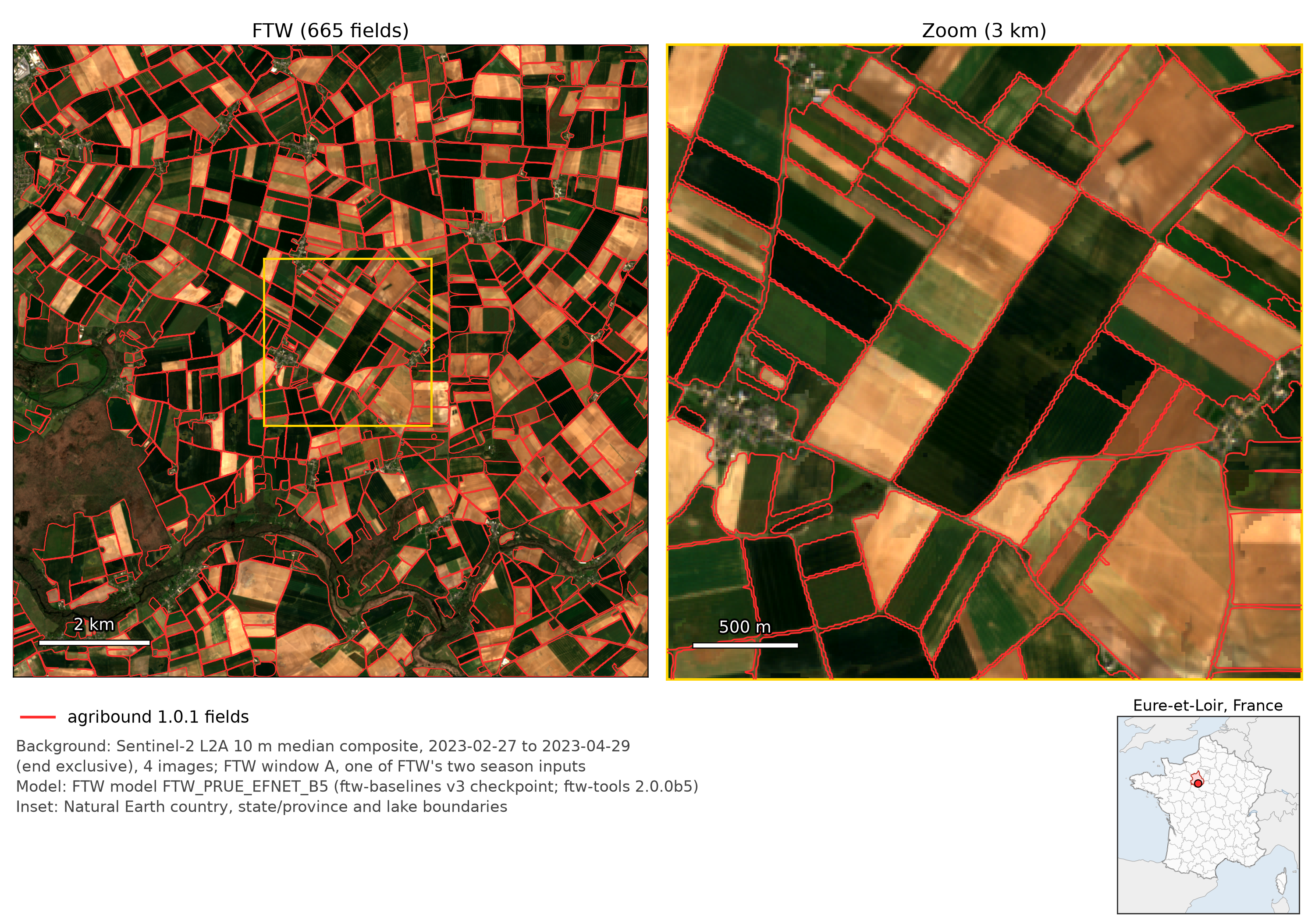
France, Beauce — FTW on Sentinel-2
Example 04 · FTW on Sentinel-2 2023 · the Beauce, Eure-et-Loir, just east of Bonneval and north-east of Châteaudun · min. area 5,000 m²; Dynamic World 2023 crop filter · FTW read two season windows chosen from the FTW crop calendar, 27 Feb–28 Apr (4 images, shown) and 7 Aug–6 Oct 2023 (4 images).
665 fields (median 10.0 ha); the crop filter kept all of them.
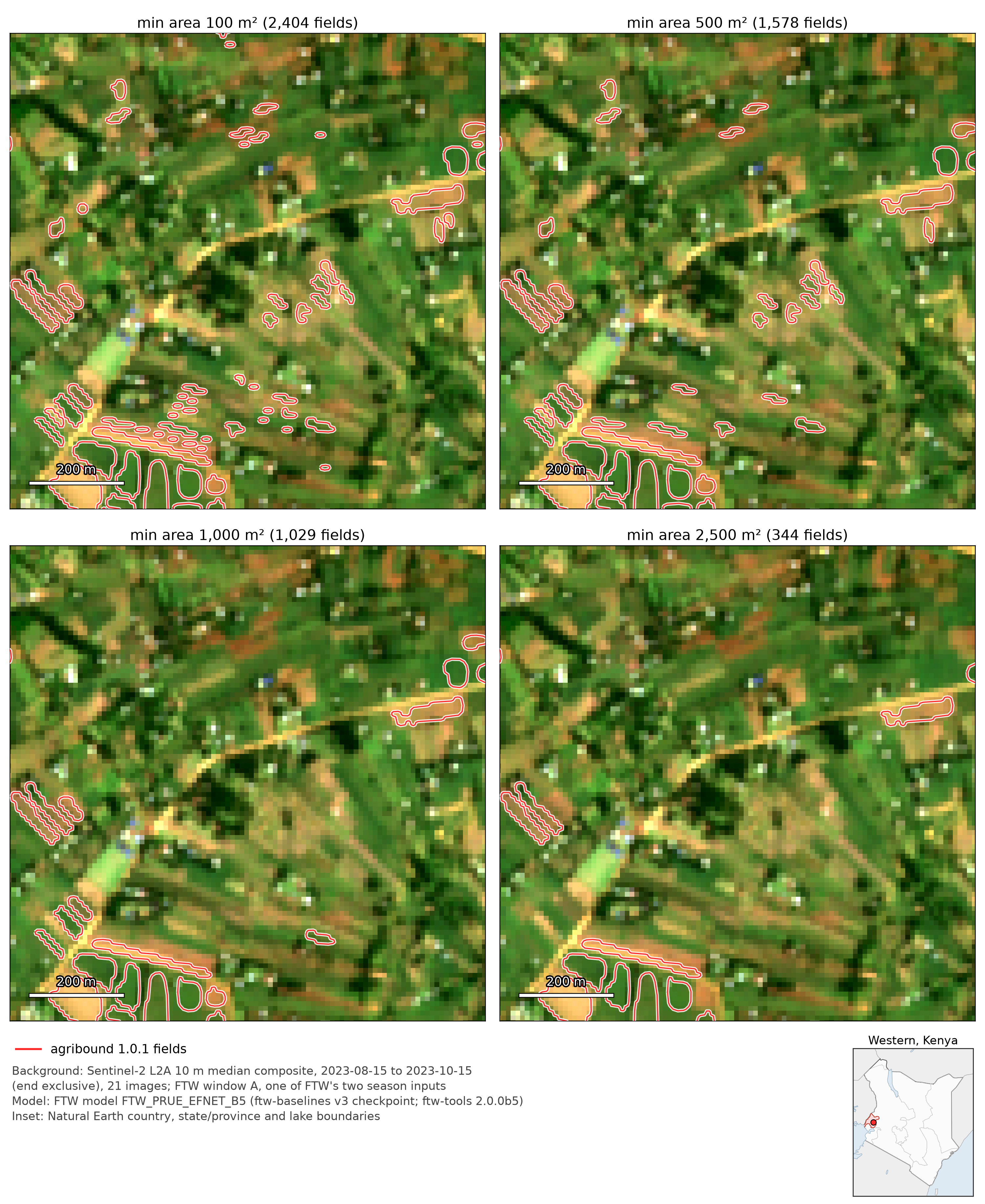
Kenya, Kakamega — FTW on Sentinel-2 at four minimum areas
Example 06 · FTW on Sentinel-2 2023 · Kakamega County, Western Kenya,
mainly Malava sub-county, an area of small farms (field sizes in this box were
not measured) · Dynamic World 2023 crop filter · FTW windows
15 Aug–14 Oct 2023 (21 images, shown) and 11 Jan–11 Mar 2024 (8 images) ·
four min_field_area_m2 values in the same 1 km window (the most polygons at
100 m²; outlines drawn with a white halo).
Fields: 2,404 at 100 m², 1,578 at 500 m², 1,029 at 1,000 m² and 344 at
2,500 m². The minimum area also applies when FTW's prediction is polygonised,
not only as a filter afterwards. The crop filter removes most of the FTW
polygons: it kept 2,404 of 24,616 at 100 m² (10 %) and 344 of 1,987 at
2,500 m² (17 %). Why they are removed was not measured, and there is no
reference layer here. Before relying on the filter in a landscape like this,
compare the output with and without it (lulc_filter,
lulc_crop_threshold).
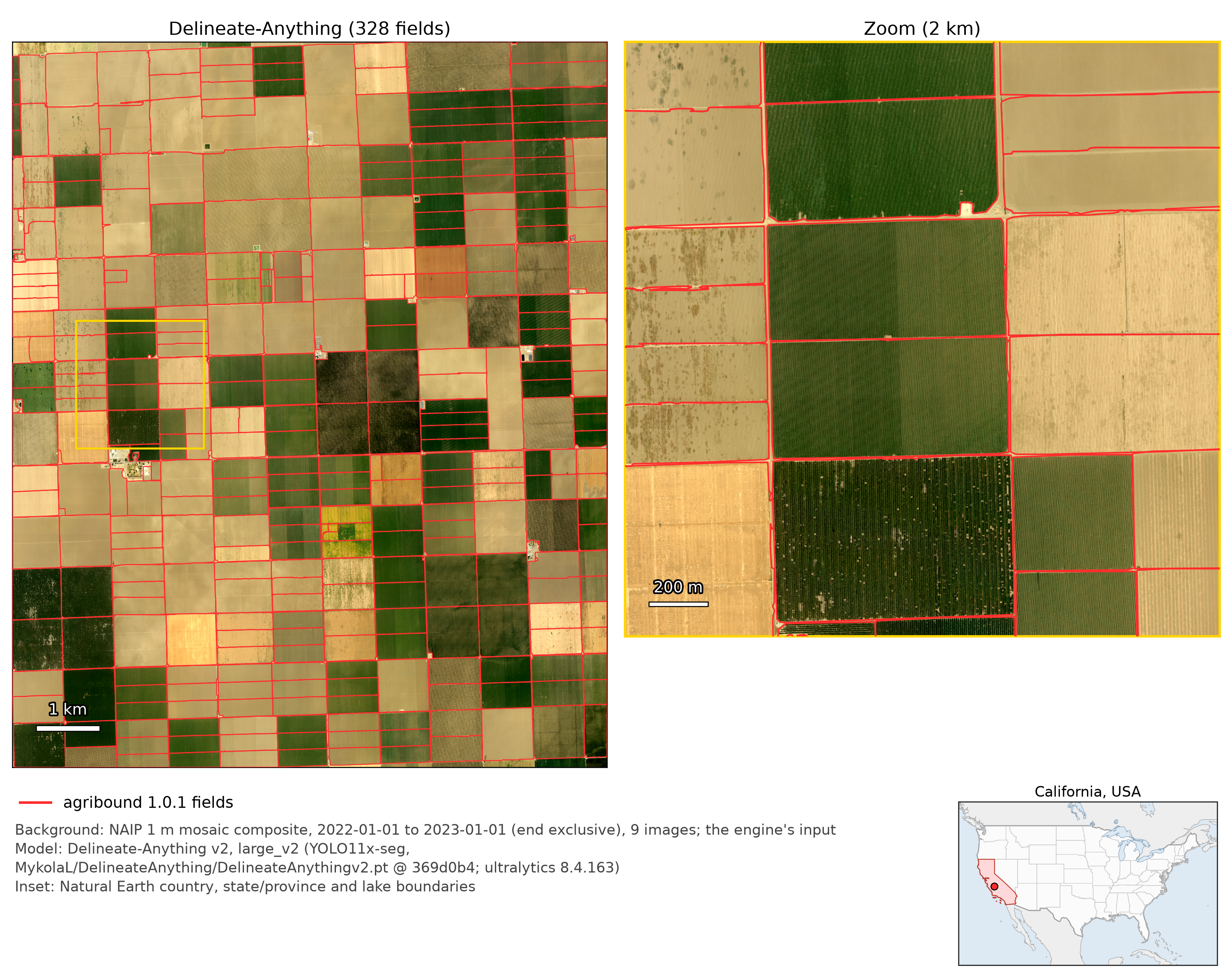
California, USA — Delineate-Anything on NAIP
Example 07 · Delineate Anything v2 on NAIP 1 m, 2022 (9 scenes, mosaicked, from Earth Engine) · western San Joaquin Valley, Fresno County, near Five Points · min. area 10,000 m²; Annual NLCD 2022 crop filter.
328 fields (median 22.6 ha); the crop filter kept all of them.
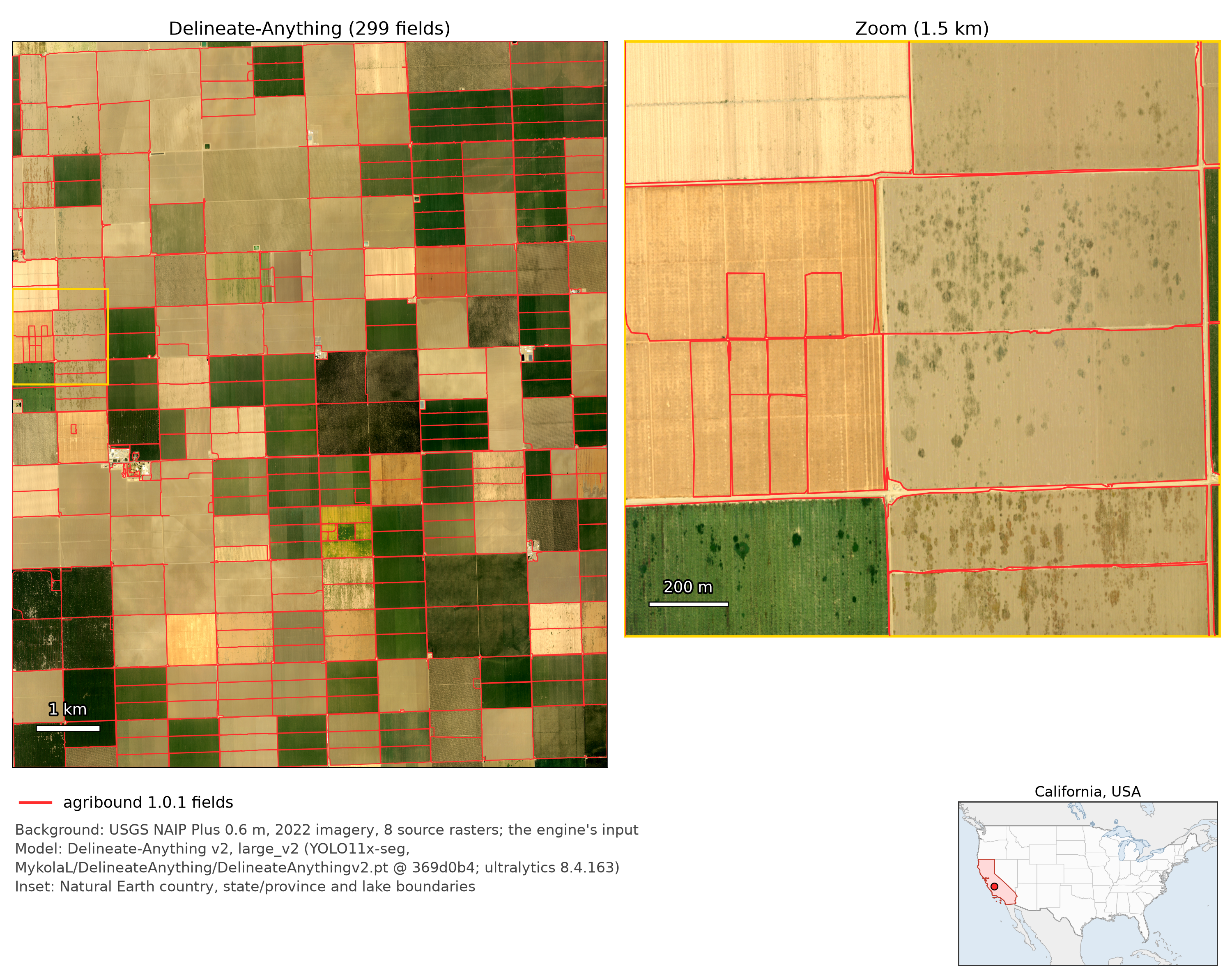
California, USA — Delineate-Anything on USGS NAIP Plus (no Earth Engine)
Example 16 · Delineate Anything v2 on USGS NAIP Plus (0.6 m, 2022; 8 source rasters exported from the USGS ImageServer) · the same study area as example 07 · min. area 10,000 m²; no crop filter.
299 fields (median 22.1 ha). This source path needs no Earth Engine, so the example runs without the crop filter, which reads its land-cover data from Earth Engine.
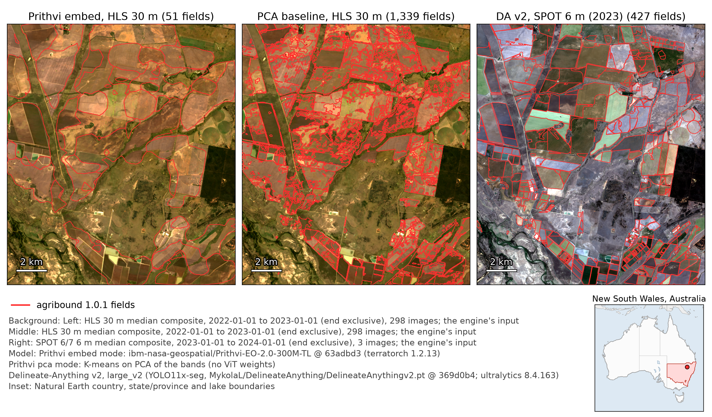
Australia, Murray-Darling Basin — Prithvi on HLS vs Delineate-Anything v2 on SPOT
Example 03 · Narrabri Shire, New South Wales, just north of Narrabri · min. area 5,000 m²; Dynamic World crop filter · the Prithvi runs use the GFM environment.
- Left: Prithvi-EO-2.0
mode="embed": K-means on the patch tokens of the last encoder layer. The tokens are 16 pixels, 480 m, apart at 30 m and are interpolated to pixels. It merges neighbouring fields into 51 polygons (median 132 ha). - Middle:
mode="pca", a baseline that uses no Prithvi weights: K-means on the PCA of per-band z-scores of R, G, B and NIR. It splits fields along within-field variation into 1,339 fragments (median 1.4 ha). - Right: Delineate Anything v2 ("DA v2") used as released, on SPOT 6/7 (6 m), 2023 (3 images; SPOT has no scene over this box in 2022): 427 fields that follow the rectangular field edges.
The left and middle panels use HLS 2022 (30 m, 298 scenes); the right panel is a year later. There is no reference layer here, so the panels compare outlines, not accuracy.
Neither mode delineates field instances; both cluster pixels into land-cover
segments, and neither was trained or fine-tuned on field boundaries in these
runs. The embed mode's over-merging, first seen in 0.1.x, remains with the
corrected HLS radiometry of 1.0. Prithvi's supervised mode="segment" needs
fine-tuning on reference polygons (fine_tune=True) and was not run here.
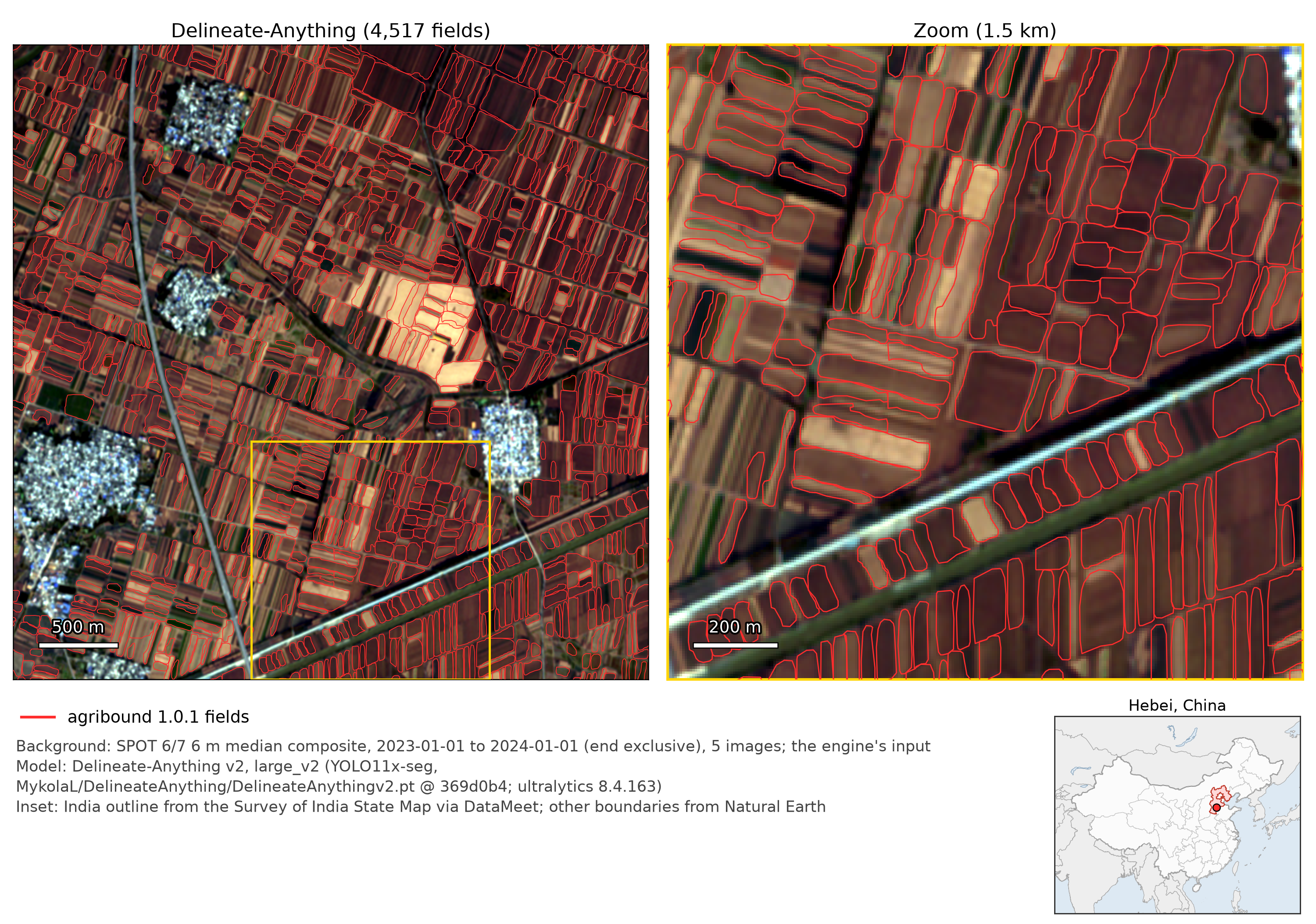
North China Plain — Delineate-Anything on SPOT
Example 08 · Delineate Anything v2 on SPOT 6/7 (6 m), 2023 (5 scenes; restricted SPOT access) · Hengshui (Jizhou District), Hebei · min. area 3,000 m²; Dynamic World 2023 crop filter · window: the 4 km square with the most Delineate-Anything polygons.
4,517 strip fields in the study area (median 0.60 ha); the crop filter kept 4,517 of 4,560.
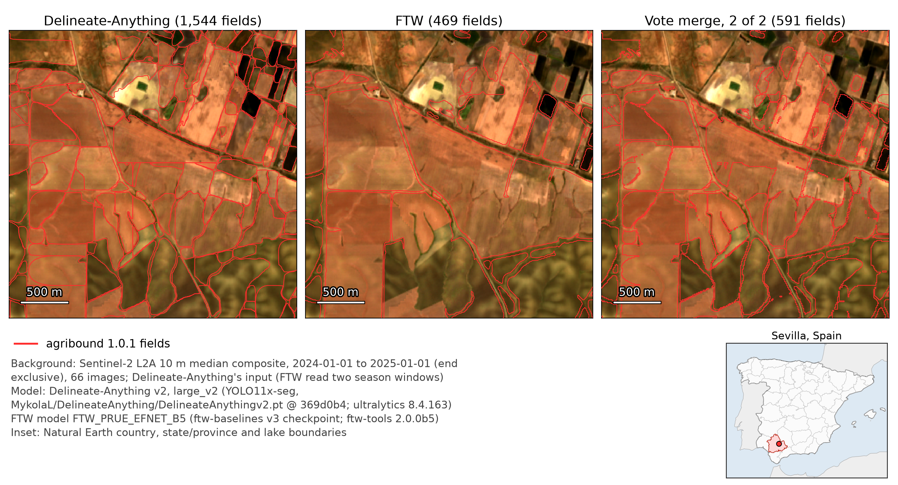
Spain, Andalusia — Delineate-Anything, FTW and their vote merge
Example 09 · Delineate Anything v2 and FTW on Sentinel-2 2024, combined afterwards from the saved outputs · Seville province, east of Carmona (the 3 km window is at the study area's east edge, in the Carmona and Fuentes de Andalucía municipalities; the most Delineate-Anything polygons) · min. area 2,500 m²; Dynamic World 2024 crop filter · Delineate-Anything read the annual composite (66 images, shown); FTW read 12 Mar–11 May and 11 Sep–10 Nov 2024 (4 images each).
Delineate-Anything returns 1,544 fields (median 4.2 ha) and FTW 469 (median 6.5 ha). The vote merge keeps the pixels that both engines cover, on a 10 m grid, which gives it its stair-stepped outlines. Neighbouring fields that are both kept fuse into one polygon: 793 polygons, 591 after the 2,500 m² filter. The example also writes the intersection (1,446) and union (695) merges, which are computed on the vector polygons.
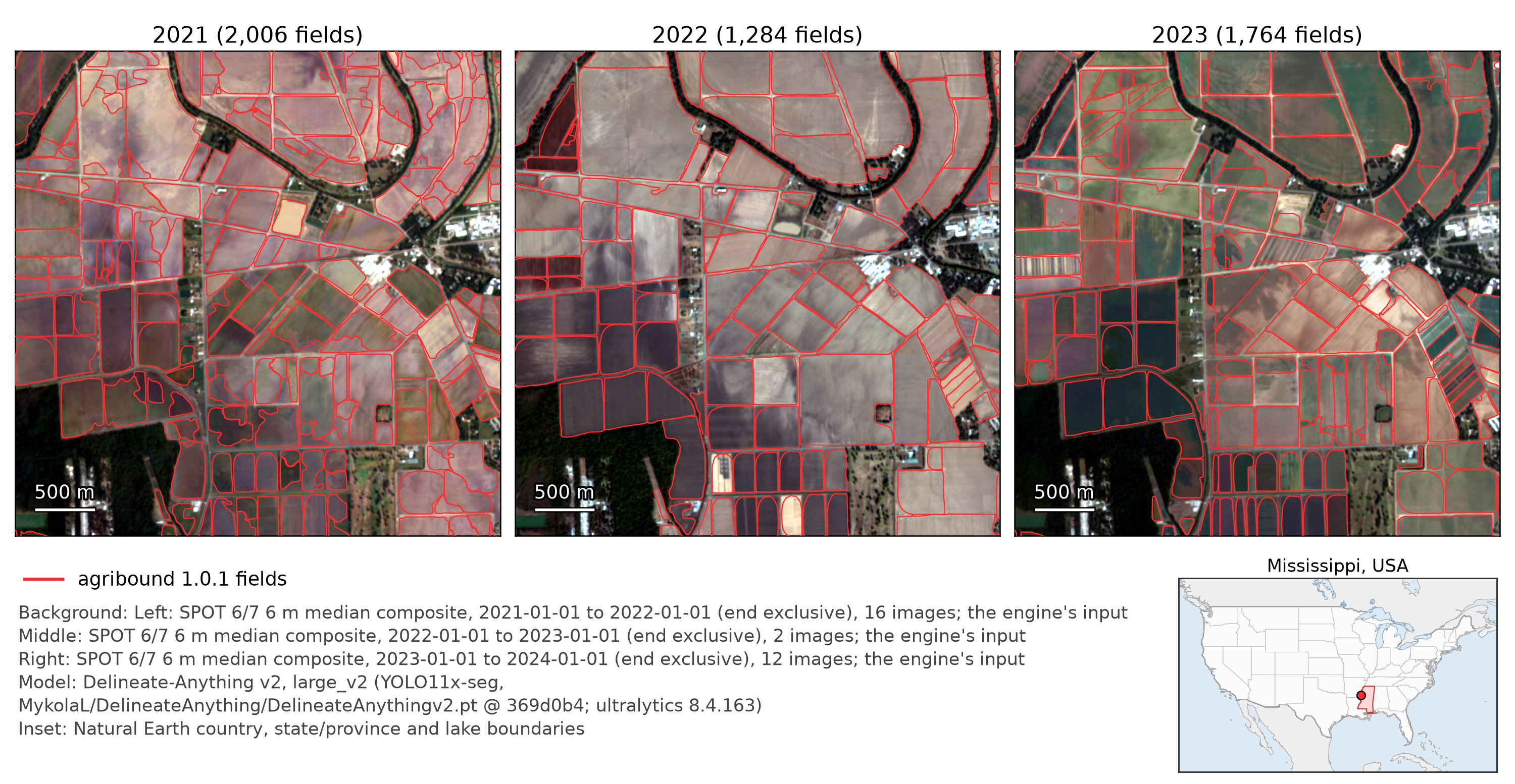
Mississippi Alluvial Plain, USA — Delineate-Anything on SPOT, 2021–2023
Example 11 · Delineate Anything v2 on SPOT 6/7 (6 m) for 2021, 2022 and 2023, each panel on its own year's composite (restricted SPOT access) · near Greenville, Washington County, Mississippi (about 6 % of the study area, in its north-western corner, is in Chicot County, Arkansas, by US Census county boundaries; the 4 km window, the square with the most 2023 polygons, centre 33.42° N, 90.93° W, is in Mississippi) · min. area 10,000 m²; Annual NLCD crop filter of each year.
2,006, 1,284 and 1,764 fields. The 2022 composite has only 2 SPOT scenes (16 in 2021, 12 in 2023). That year has the fewest polygons and the largest median area (7.8 ha, against 4.2 and 5.0 ha), while the total delineated area is similar; these runs do not test whether the scene count is the cause. Year-to-year agreement (one-to-one matching at IoU ≥ 0.5) is F1 0.49 from 2021 to 2022 and 0.55 from 2022 to 2023; this compares predictions with each other and says nothing about accuracy.
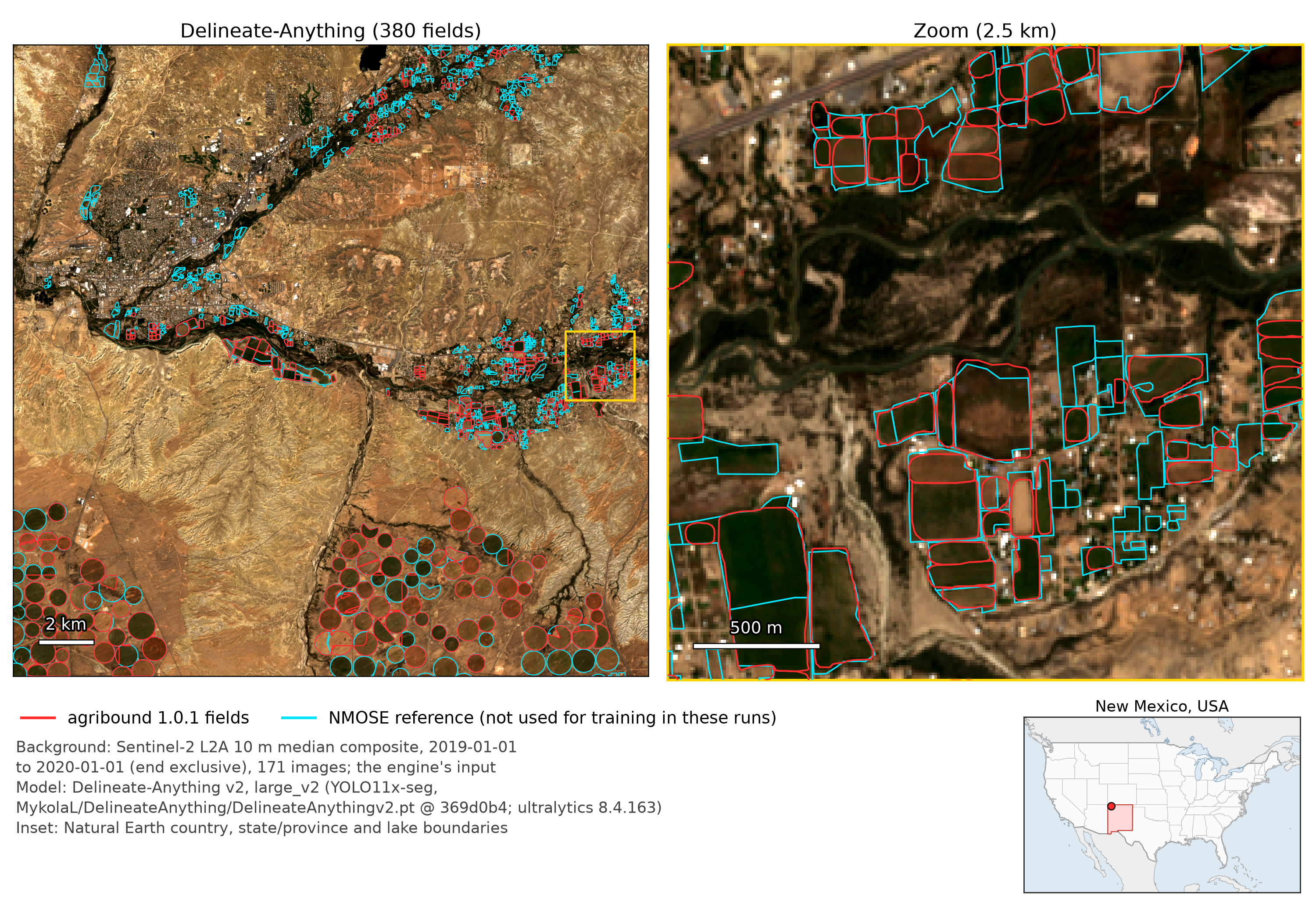
San Juan County, New Mexico — evaluation against NMOSE
Example 20 · Delineate Anything v2 on Sentinel-2 2019 (171 images) · San Juan County, New Mexico (Farmington–Bloomfield area) · min. area 2,500 m²; Annual NLCD 2019 crop filter · evaluated against the NMOSE WUCB polygons (cyan), which were not used for training or fine-tuning in these runs (Delineate Anything v2 is used as released; whether its training set, FBIS-73M, includes them was not checked).
Of the 380 predictions, 379 lie inside the evaluation box (by representative point; the panel title counts all 380, and the other one lies across the box's south edge), against 944 reference fields. One-to-one matching at IoU ≥ 0.5 gives precision 0.58, recall 0.23 and F1 0.33 (95 % bootstrap intervals from 200 resamples of reference fields within sub-basins: F1 0.31–0.36, recall 0.21–0.25; they treat fields as independent, so they are too narrow if errors are spatially clustered); the mean IoU of matched fields is 0.80. Area-weighted recall is 0.61 and area-weighted precision 0.84. Recall rises with field size and then levels off: it is 0.01 for fields of 0.2–0.5 ha and about 0.7 for fields above 10 ha. F1 broadly follows but dips at 5–10 ha (0.32, against 0.41 at 2–5 ha) and at 50–100 ha (0.59, against 0.69 at 20–50 ha). By sub-basin, NIIP (the Navajo Indian Irrigation Project; 97 reference fields, all 18 ha or larger) reaches F1 0.72, and the Animas River (324 reference fields, median 0.83 ha) F1 0.18. Two caveats: the reference was digitised from 2016 NAIP, so changes by 2019 count as errors, and the crop filter removed 182 of 562 polygons before the evaluation.
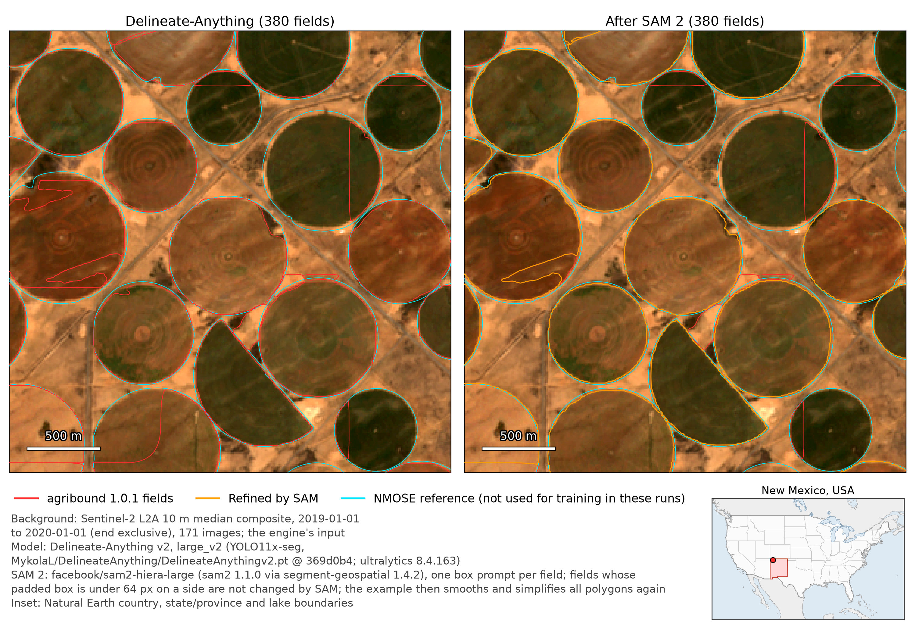
SAM 2 refinement — example 20's output before and after
Example 13 · SAM 2 box-prompted refinement of example 20's Delineate-Anything output (Sentinel-2 2019). The default input of this example is example 12's output, which was not run for 1.0.0 or 1.0.1 · window: the most SAM-refined fields, the centre pivots of the Navajo Indian Irrigation Project, San Juan County.
At 10 m, only 67 of the 380 fields pass the SAM size rule (all 19 ha or
larger); the other 313 are not refined. After SAM, the example smooths
(Chaikin ×3) and simplifies all 380 polygons again, although example 20's
output was already smoothed, so the before/after numbers include this second
smoothing. Against the NMOSE polygons, object F1 is unchanged (0.332, 220
matches before and after), and the mean boundary distance falls from 13.4 m
to 12.5 m, with SAM and the second smoothing together. SAM replaces each
prompted polygon with its own mask and never merges or deletes polygons
(380 in, 380 out), so Delineate-Anything's splits inside pivots remain; with
sam_overlaps="trim" a refined mask also cannot take area from a
neighbouring polygon (14 masks were trimmed). Every mask covered at least
92 % of its polygon, so the coverage test of 1.0.1 (sam_min_coverage = 0.5)
rejected none (covering too little: 0), and the 1.0.1 output is identical to
the 1.0.0 one. (Example 13 evaluates all 380 polygons; example 20 evaluates
the 379 inside its box.)
HPC tiling — four tiles merged
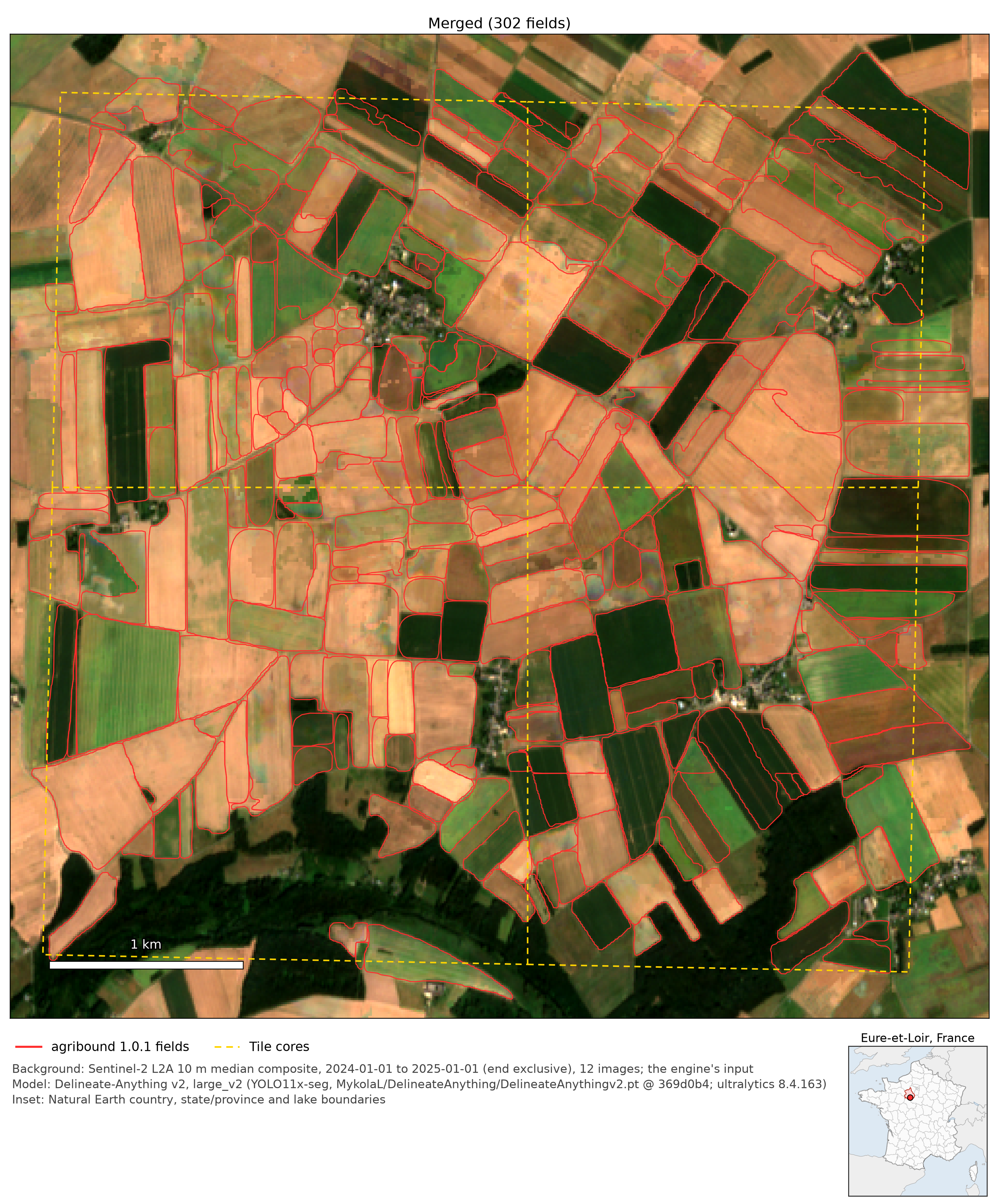
Example 19 · the agribound.hpc workflow (make tiles, run, merge) run
locally on a 4.5 × 4.5 km study area in the Beauce, Eure-et-Loir, east of
Bonneval (inside example 04's study area) · Delineate Anything v2 on
Sentinel-2 2024 composites, one per tile · min. area 2,500 m²; Dynamic World
2024 crop filter.
The study area is cut along the UTM 31N grid into four core tiles of up to 2.5 km (dashed); their outer edges follow the study area's longitude/latitude box, so they lean slightly in this UTM view. Each core is delineated with a 1 km halo around it. The merge keeps each polygon only in the tile that owns its representative point: 1,177 tile polygons become 302. No polygon reached a halo edge, so fields that cross the core edges come out whole; one field was delineated by two tiles and appears twice (the pair is not marked).