Water-Table Depth Interpolation

pyGWRetrieval can turn point water-level observations into gridded water-table depth maps for a chosen temporal window, at a resolution you specify in meters. This guide covers the typical workflow; see the API Reference for full signatures.

Installation

Interpolation uses optional dependencies:

pip install pyGWRetrieval[interp]   # scipy, pykrige, rasterio, xarray

IDW works with the core install; kriging needs pykrige, and linear/cubic/nearest/rbf need scipy. GeoTIFF/xarray export need rasterio/xarray.

Methods

Method	Notes
idw	Inverse distance weighting (pure NumPy, always available)
kriging	Ordinary kriging (pykrige)
linear / cubic	Delaunay-based; only fill the convex hull of the wells (see fill_outside)
nearest	Nearest-neighbor (Voronoi cells)
rbf	Radial basis function / thin-plate spline (can overshoot when extrapolating)

Workflow

from pyGWRetrieval import GroundwaterRetrieval, WaterTableInterpolator
from pyGWRetrieval.spatial import get_geometry_from_shapefile, merge_geometries

# 1. Retrieve field measurements + daily values for an area of interest.
gw = GroundwaterRetrieval(start_date='1985-01-01', data_sources=['gwlevels', 'dv'])
data = gw.get_data_by_shapefile('basin.shp')

# 2. Keep depth-to-water only (parameter 72019) so wells are comparable.
depth = data[data['parameter_cd'] == '72019']

# 3. Restrict to unconfined (water-table) aquifer wells. Discovery already
#    attached aqfr_type_cd to gw.wells.
unconfined = set(gw.wells.loc[gw.wells['aqfr_type_cd'] == 'U', 'site_no'])
wtd = depth[depth['site_no'].isin(unconfined)]

# 4. Interpolate to a 1 km grid, clipped to the basin.
basin = merge_geometries(get_geometry_from_shapefile('basin.shp'))
interp = WaterTableInterpolator(wtd, value_column='lev_va', date_column='datetime')
grids = interp.interpolate(period='all', method='idw', grid_size_m=1000, boundary=basin)

# 5. Export.
result = grids['all']
result.to_geotiff('wtd_mean_idw.tif')   # also result.plot() and result.to_xarray()

interpolate() returns a dict of window label → InterpolationResult. Use period='monthly' / 'annual' / 'custom' for time-resolved maps.

Method comparison

The Upper Colorado River Basin example builds a long-term mean water-table depth map (1985-present, 1 km grid) and compares the methods on the same well set:

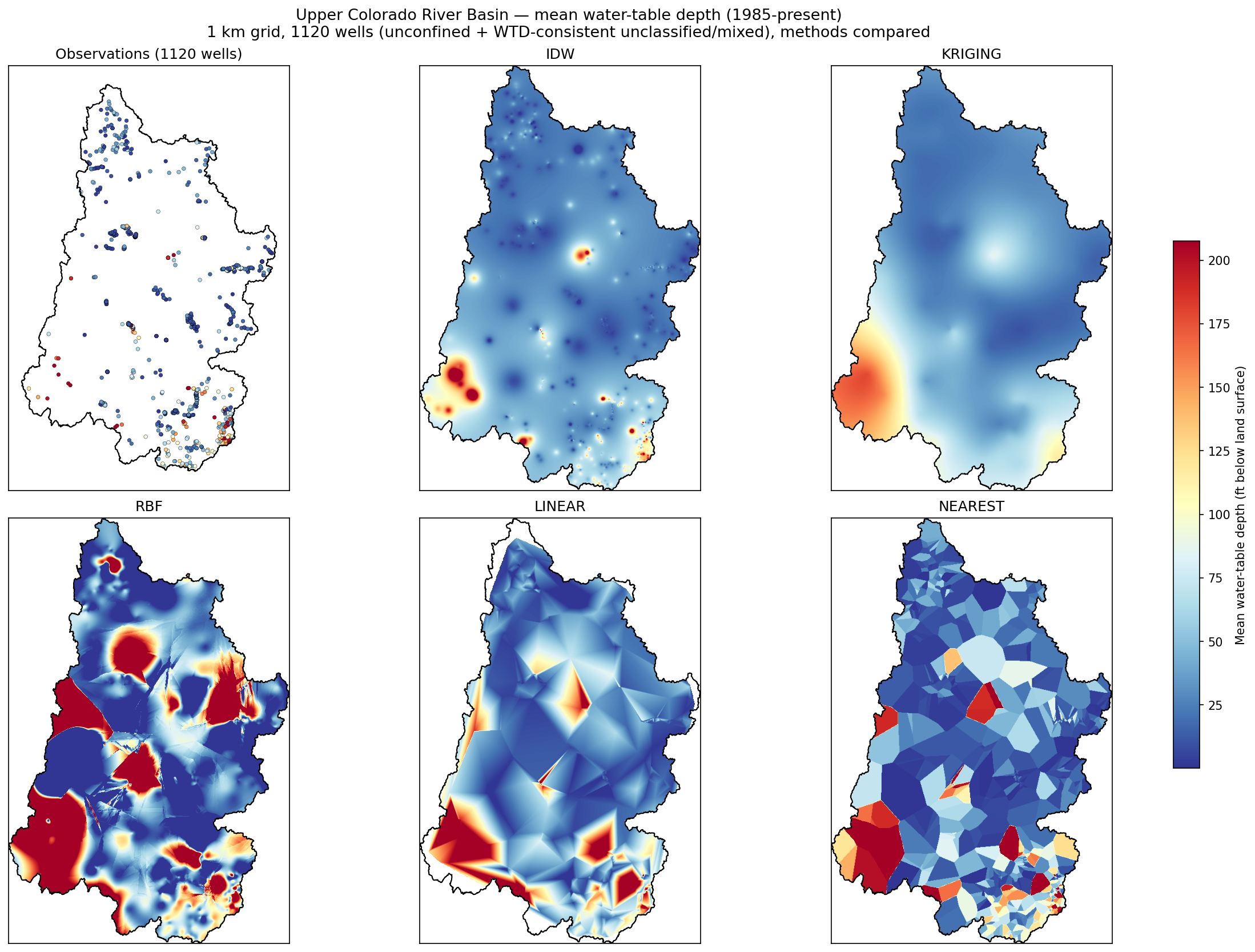
IDW produces smooth bullseyes around wells; kriging a smooth geostatistical surface; RBF fits tightly but overshoots when extrapolating; linear only fills the Delaunay hull of the points; nearest yields hard Voronoi cells.

Full basin coverage for Delaunay methods

linear and cubic do not extrapolate beyond the wells' convex hull (cells outside it are NaN). Backfill them with a secondary method:

interp.interpolate(period='all', method='linear', grid_size_m=1000,
                   boundary=basin, fill_outside='nearest')

Choosing a resolution

grid_size_m sets the cell size in meters; observations are projected to a metric CRS (auto-UTM by default) before interpolation. Match the resolution to your well density and extent — a very fine grid over a large, sparsely-monitored area is neither tractable nor statistically meaningful.

Point estimates and cross-validation

idw_at_points estimates at arbitrary scattered locations (not a grid), with an optional leave-one-out mode for cross-validation — useful, for example, to keep unclassified wells whose depth-to-water is consistent with the surface defined by confirmed unconfined wells. How inclusive that consistency test is (an acceptance band on the leave-one-out residuals) trades coverage against confidence, but the regional pattern is stable:

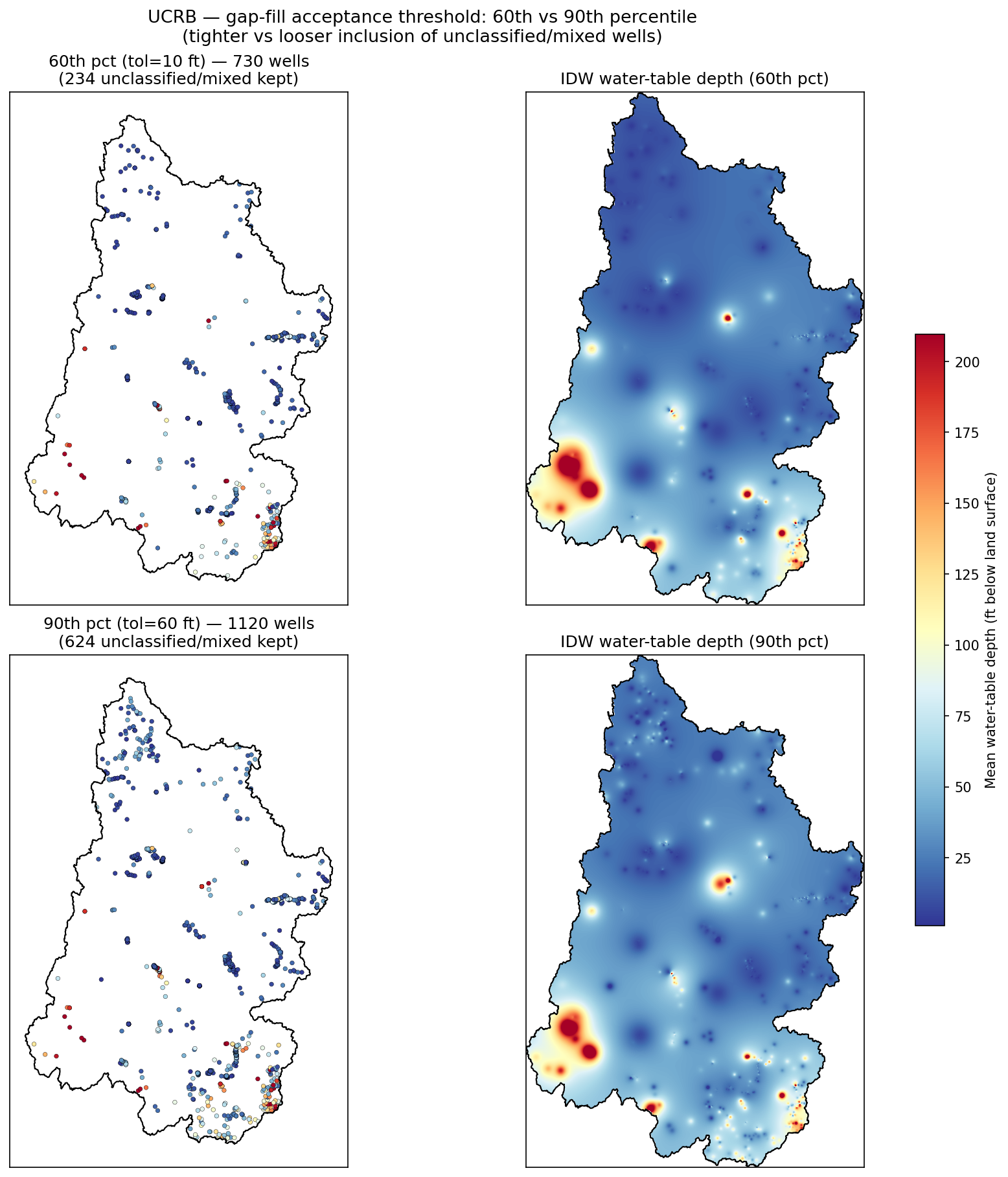
See the Upper Colorado River Basin example for the full workflow.