Examples
Example 1: ERA5-Land for South America
Calculate effective precipitation for a large river basin using ERA5-Land monthly data.
Python:
from pycropwat import EffectivePrecipitation

ep = EffectivePrecipitation(
    asset_id='ECMWF/ERA5_LAND/MONTHLY_AGGR',
    precip_band='total_precipitation_sum',
    gee_geometry_asset='projects/my-project/assets/amazon_basin',
    start_year=2010,
    end_year=2023,
    precip_scale_factor=1000  # ERA5 precipitation is in meters
)

results = ep.process(
    output_dir='./amazon_effective_precip',
    n_workers=8
)
CLI:
pycropwat process \
    --asset ECMWF/ERA5_LAND/MONTHLY_AGGR \
    --band total_precipitation_sum \
    --gee-geometry projects/my-project/assets/amazon_basin \
    --start-year 2010 \
    --end-year 2023 \
    --scale-factor 1000 \
    --workers 8 \
    --output ./amazon_effective_precip
Example 2: TerraClimate Long-term Analysis
Process 40+ years of TerraClimate data for drought analysis.
Python:
from pycropwat import EffectivePrecipitation

ep = EffectivePrecipitation(
    asset_id='IDAHO_EPSCOR/TERRACLIMATE',
    precip_band='pr',
    geometry_path='western_us.geojson',
    start_year=1980,
    end_year=2023
    # No scale_factor needed - TerraClimate is already in mm
)

# Process only growing season months
results = ep.process(
    output_dir='./terraclimate_growing_season',
    n_workers=4,
    months=[4, 5, 6, 7, 8, 9, 10]  # April-October
)
CLI:
pycropwat process \
    --asset IDAHO_EPSCOR/TERRACLIMATE \
    --band pr \
    --geometry western_us.geojson \
    --start-year 1980 \
    --end-year 2023 \
    --months 4 5 6 7 8 9 10 \
    --workers 4 \
    --output ./terraclimate_growing_season
Example 3: High-Resolution Custom Output
Generate 1km resolution outputs from ERA5-Land.
Python:
from pycropwat import EffectivePrecipitation

ep = EffectivePrecipitation(
    asset_id='ECMWF/ERA5_LAND/MONTHLY_AGGR',
    precip_band='total_precipitation_sum',
    geometry_path='small_watershed.geojson',
    start_year=2020,
    end_year=2023,
    scale=1000,  # 1 km resolution
    precip_scale_factor=1000
)

results = ep.process(output_dir='./high_res_outputs', n_workers=4)
CLI:
pycropwat process \
    --asset ECMWF/ERA5_LAND/MONTHLY_AGGR \
    --band total_precipitation_sum \
    --geometry small_watershed.geojson \
    --start-year 2020 \
    --end-year 2023 \
    --scale 1000 \
    --scale-factor 1000 \
    --output ./high_res_outputs
Example 4: CHIRPS for Africa
Use CHIRPS daily data for African agriculture analysis.
Python:
from pycropwat import EffectivePrecipitation

ep = EffectivePrecipitation(
    asset_id='UCSB-CHG/CHIRPS/DAILY',
    precip_band='precipitation',
    gee_geometry_asset='projects/my-project/assets/africa_croplands',
    start_year=2015,
    end_year=2023
)

results = ep.process(
    output_dir='./africa_chirps_outputs',
    n_workers=8,
    months=[3, 4, 5, 6, 7, 8, 9, 10]  # Growing season
)
CLI:
pycropwat process \
    --asset UCSB-CHG/CHIRPS/DAILY \
    --band precipitation \
    --gee-geometry projects/my-project/assets/africa_croplands \
    --start-year 2015 \
    --end-year 2023 \
    --months 3 4 5 6 7 8 9 10 \
    --workers 8 \
    --output ./africa_chirps_outputs
Note
Daily CHIRPS data is automatically summed to monthly totals.
Example 5: Using Different Peff Methods
Compare different effective precipitation methods.
Python:
from pycropwat import EffectivePrecipitation
from pycropwat.methods import (
    cropwat_effective_precip,
    fao_aglw_effective_precip,
    fixed_percentage_effective_precip,
    dependable_rainfall_effective_precip
)
import numpy as np

# Direct calculation with numpy arrays
precip = np.array([50, 100, 150, 200, 250, 300])

print("Monthly Precip:", precip)
print("CROPWAT:", cropwat_effective_precip(precip))
print("FAO/AGLW:", fao_aglw_effective_precip(precip))
print("Fixed 80%:", fixed_percentage_effective_precip(precip, 0.8))
print("Depend 75%:", dependable_rainfall_effective_precip(precip, 0.75))
CLI:
# CROPWAT method
pycropwat process --asset IDAHO_EPSCOR/TERRACLIMATE --band pr \
    --geometry roi.geojson --start-year 2015 --end-year 2020 \
    --method cropwat --output ./output_cropwat

# FAO/AGLW method
pycropwat process --asset IDAHO_EPSCOR/TERRACLIMATE --band pr \
    --geometry roi.geojson --start-year 2015 --end-year 2020 \
    --method fao_aglw --output ./output_fao

# Fixed percentage (80%)
pycropwat process --asset IDAHO_EPSCOR/TERRACLIMATE --band pr \
    --geometry roi.geojson --start-year 2015 --end-year 2020 \
    --method fixed_percentage --percentage 0.8 --output ./output_fixed

# Dependable rainfall (80% probability)
pycropwat process --asset IDAHO_EPSCOR/TERRACLIMATE --band pr \
    --geometry roi.geojson --start-year 2015 --end-year 2020 \
    --method dependable_rainfall --probability 0.8 --output ./output_depend
Example 6: Temporal Aggregation
Aggregate monthly data into seasonal, annual, and climatology products.
Python:
from pycropwat.analysis import TemporalAggregator

agg = TemporalAggregator('./outputs')

# Annual totals for each year
for year in range(2010, 2024):
    agg.annual_aggregate(
        year=year,
        method='sum',
        output_path=f'./annual/annual_{year}.tif'
    )

# Seasonal aggregations
for year in range(2010, 2024):
    for season in ['DJF', 'MAM', 'JJA', 'SON']:
        agg.seasonal_aggregate(
            year=year,
            season=season,
            method='sum',
            output_path=f'./seasonal/{season}_{year}.tif'
        )

# Growing season - Northern Hemisphere (April-October)
for year in range(2010, 2024):
    agg.growing_season_aggregate(
        year=year,
        start_month=4,
        end_month=10,
        method='sum',
        output_path=f'./growing/growing_{year}.tif'
    )

# Growing season - Southern Hemisphere (October-March, cross-year)
# When start_month > end_month, automatically spans two calendar years
for year in range(2010, 2023):  # End at 2023 since we need data from year+1
    agg.growing_season_aggregate(
        year=year,
        start_month=10,  # October
        end_month=3,     # March (of year+1)
        method='sum',
        output_path=f'./growing/growing_{year}_{year+1}.tif'
    )

# 30-year climatology (long-term monthly means)
climatology = agg.climatology(
    start_year=1990,
    end_year=2020,
    method='mean',
    output_dir='./climatology/'
)
CLI:
# Annual total
pycropwat aggregate --input ./outputs --type annual \
    --year 2020 --output ./annual_2020.tif

# Summer (JJA) aggregate
pycropwat aggregate --input ./outputs --type seasonal \
    --year 2020 --season JJA --output ./summer_2020.tif

# Growing season (April-October)
pycropwat aggregate --input ./outputs --type growing-season \
    --year 2020 --start-month 4 --end-month 10 \
    --output ./growing_2020.tif

# 30-year climatology
pycropwat aggregate --input ./outputs --type climatology \
    --start-year 1990 --end-year 2020 --output ./climatology/
Example 7: Statistical Analysis
Perform anomaly detection, trend analysis, and zonal statistics.
Python:
from pycropwat.analysis import TemporalAggregator, StatisticalAnalyzer

agg = TemporalAggregator('./outputs')
stats = StatisticalAnalyzer(agg)

# Percent anomaly for June 2023 relative to 1990-2020 climatology
anomaly = stats.calculate_anomaly(
    year=2023,
    month=6,
    clim_start=1990,
    clim_end=2020,
    anomaly_type='percent',
    output_path='./anomaly_2023_06.tif'
)

# Standardized anomaly (z-score)
anomaly_std = stats.calculate_anomaly(
    year=2023,
    month=6,
    clim_start=1990,
    clim_end=2020,
    anomaly_type='standardized',
    output_path='./anomaly_std_2023_06.tif'
)

# Linear trend analysis (2000-2020)
trend = stats.calculate_trend(
    start_year=2000,
    end_year=2020,
    method='linear',
    output_dir='./trend_linear/'
)
print(f"Trend outputs: slope, intercept, r_squared, p_value")

# Theil-Sen trend with Mann-Kendall test
trend_sen = stats.calculate_trend(
    start_year=2000,
    end_year=2020,
    method='sen',
    output_dir='./trend_sen/'
)

# Zonal statistics by administrative region
zonal_df = stats.zonal_statistics(
    geometry_path='./admin_regions.shp',
    start_year=2010,
    end_year=2020,
    stats=['mean', 'sum', 'min', 'max', 'std'],
    output_path='./zonal_stats.csv'
)
print(zonal_df.head())
CLI:
# Percent anomaly
pycropwat analyze anomaly --input ./outputs \
    --year 2023 --month 6 \
    --clim-start 1990 --clim-end 2020 \
    --anomaly-type percent \
    --output ./anomaly_2023_06.tif

# Theil-Sen trend analysis
pycropwat analyze trend --input ./outputs \
    --start-year 2000 --end-year 2020 \
    --trend-method sen \
    --output ./trend/

# Zonal statistics
pycropwat analyze zonal --input ./outputs \
    --zones ./admin_regions.shp \
    --start-year 2010 --end-year 2020 \
    --output ./zonal_stats.csv
Example 8: Export to Different Formats
Export data to NetCDF and Cloud-Optimized GeoTIFF.
Python:
from pycropwat.analysis import export_to_netcdf, export_to_cog
from pathlib import Path

# Export all monthly data to a single NetCDF file
export_to_netcdf(
    input_dir='./outputs',
    output_path='./effective_precip.nc',
    variable_name='effective_precip',
    pattern='effective_precip_[0-9]*.tif',  # Excludes fraction files
    compression=True
)

# Batch convert to Cloud-Optimized GeoTIFFs (excludes fraction files)
output_cog_dir = Path('./cogs')
output_cog_dir.mkdir(exist_ok=True)

for tif in Path('./outputs').glob('effective_precip_[0-9]*.tif'):
    export_to_cog(
        input_path=str(tif),
        output_path=str(output_cog_dir / tif.name)
    )
CLI:
# Export to NetCDF
pycropwat export netcdf --input ./outputs --output ./effective_precip.nc

# Convert single file to COG
pycropwat export cog \
    --input ./outputs/effective_precip_2020_06.tif \
    --output ./cogs/effective_precip_2020_06.tif

# Batch convert with shell loop (excludes fraction files)
mkdir -p ./cogs
for f in ./outputs/effective_precip_[0-9]*.tif; do
    pycropwat export cog --input "$f" --output "./cogs/$(basename $f)"
done
Example 9: Visualization
Create static plots and interactive maps.
Python:
from pycropwat.analysis import Visualizer

viz = Visualizer('./outputs')

# Time series plot
fig = viz.plot_time_series(
    start_year=2000,
    end_year=2023,
    stat='mean',
    title='Mean Effective Precipitation (2000-2023)',
    figsize=(14, 6),
    output_path='./timeseries.png'
)

# Monthly climatology bar chart
fig = viz.plot_monthly_climatology(
    start_year=2000,
    end_year=2023,
    stat='mean',
    title='Monthly Climatology (2000-2023)',
    output_path='./climatology.png'
)

# Single month raster map
fig = viz.plot_raster(
    year=2020,
    month=6,
    cmap='YlGnBu',
    vmin=0,
    vmax=150,
    title='Effective Precipitation - June 2020',
    output_path='./map_2020_06.png'
)

# Interactive map (requires: pip install leafmap)
viz.plot_interactive_map(
    year=2020,
    month=6,
    cmap='YlGnBu',
    opacity=0.7,
    zoom_start=6,
    output_path='./interactive_map.html'
)

# Anomaly map from GeoTIFF (diverging colormap, centered at 100%)
fig = viz.plot_anomaly_map(
    anomaly_path='./analysis_outputs/anomalies/ERA5Land/anomaly_2023_08.tif',
    title='Peff Anomaly - August 2023 (% of Climatology)',
    output_path='./anomaly_map_2023_08.png'
)

# Climatology map from GeoTIFF
fig = viz.plot_climatology_map(
    climatology_path='./analysis_outputs/climatology/ERA5Land/climatology_06.tif',
    title='Peff Climatology - June (2000-2020)',
    output_path='./climatology_map_06.png'
)

# Trend map with significance stippling
fig = viz.plot_trend_map(
    slope_path='./analysis_outputs/trend/ERA5Land/slope.tif',
    pvalue_path='./analysis_outputs/trend/ERA5Land/pvalue.tif',
    title='Peff Trend (2000-2023)',
    show_significance=True,  # Adds stippling for p < 0.05
    output_path='./trend_map.png'
)

# Trend panel (slope and p-value side-by-side)
fig = viz.plot_trend_panel(
    slope_path='./analysis_outputs/trend/ERA5Land/slope.tif',
    pvalue_path='./analysis_outputs/trend/ERA5Land/pvalue.tif',
    title='Peff Trend Analysis (2000-2023)',
    output_path='./trend_panel.png'
)
CLI:
# Time series plot
pycropwat plot timeseries --input ./outputs \
    --start-year 2000 --end-year 2023 \
    --title "Mean Effective Precipitation (2000-2023)" \
    --output ./timeseries.png

# Monthly climatology
pycropwat plot climatology --input ./outputs \
    --start-year 2000 --end-year 2023 \
    --output ./climatology.png

# Raster map
pycropwat plot map --input ./outputs \
    --year 2020 --month 6 \
    --cmap YlGnBu --vmin 0 --vmax 150 \
    --output ./map_2020_06.png

# Interactive map
pycropwat plot interactive --input ./outputs \
    --year 2020 --month 6 \
    --output ./interactive_map.html
Example 10: Comparing Datasets
Compare ERA5-Land vs TerraClimate effective precipitation.
Python:
from pycropwat import EffectivePrecipitation
from pycropwat.analysis import Visualizer

# Process ERA5-Land
ep_era5 = EffectivePrecipitation(
    asset_id='ECMWF/ERA5_LAND/MONTHLY_AGGR',
    precip_band='total_precipitation_sum',
    geometry_path='study_area.geojson',
    start_year=2000,
    end_year=2020,
    precip_scale_factor=1000
)
ep_era5.process(output_dir='./era5_outputs', n_workers=4)

# Process TerraClimate
ep_tc = EffectivePrecipitation(
    asset_id='IDAHO_EPSCOR/TERRACLIMATE',
    precip_band='pr',
    geometry_path='study_area.geojson',
    start_year=2000,
    end_year=2020
)
ep_tc.process(output_dir='./terraclimate_outputs', n_workers=4)

# Compare the outputs
viz = Visualizer('./era5_outputs')

# Side-by-side comparison with difference map
fig = viz.plot_comparison(
    other_dir='./terraclimate_outputs',
    year=2020,
    month=6,
    labels=('ERA5-Land', 'TerraClimate'),
    cmap='YlGnBu',
    diff_cmap='RdBu',
    output_path='./comparison_2020_06.png'
)

# Scatter plot with statistics (R², RMSE, bias)
fig = viz.plot_scatter_comparison(
    other_dir='./terraclimate_outputs',
    start_year=2000,
    end_year=2020,
    sample_size=10000,
    labels=('ERA5-Land (mm)', 'TerraClimate (mm)'),
    output_path='./scatter_comparison.png'
)

# Annual totals comparison
fig = viz.plot_annual_comparison(
    other_dir='./terraclimate_outputs',
    start_year=2000,
    end_year=2020,
    labels=('ERA5-Land', 'TerraClimate'),
    output_path='./annual_comparison.png'
)
CLI:
# Process both datasets
pycropwat process --asset ECMWF/ERA5_LAND/MONTHLY_AGGR \
    --band total_precipitation_sum \
    --geometry study_area.geojson \
    --start-year 2000 --end-year 2020 \
    --scale-factor 1000 --output ./era5_outputs

pycropwat process --asset IDAHO_EPSCOR/TERRACLIMATE \
    --band pr \
    --geometry study_area.geojson \
    --start-year 2000 --end-year 2020 \
    --output ./terraclimate_outputs

# Side-by-side comparison
pycropwat plot compare \
    --input ./era5_outputs \
    --other-input ./terraclimate_outputs \
    --year 2020 --month 6 \
    --label1 ERA5-Land --label2 TerraClimate \
    --output ./comparison_2020_06.png

# Scatter plot
pycropwat plot scatter \
    --input ./era5_outputs \
    --other-input ./terraclimate_outputs \
    --start-year 2000 --end-year 2020 \
    --output ./scatter_comparison.png

# Annual comparison
pycropwat plot annual-compare \
    --input ./era5_outputs \
    --other-input ./terraclimate_outputs \
    --start-year 2000 --end-year 2020 \
    --label1 ERA5-Land --label2 TerraClimate \
    --output ./annual_comparison.png
Example 11: Batch Processing Multiple Regions
Python:
from pycropwat import EffectivePrecipitation
from pathlib import Path

regions = [
    'projects/my-project/assets/region_north',
    'projects/my-project/assets/region_south',
    'projects/my-project/assets/region_east',
    'projects/my-project/assets/region_west',
]

for region in regions:
    region_name = region.split('/')[-1]
    print(f"Processing {region_name}...")

    ep = EffectivePrecipitation(
        asset_id='ECMWF/ERA5_LAND/MONTHLY_AGGR',
        precip_band='total_precipitation_sum',
        gee_geometry_asset=region,
        start_year=2020,
        end_year=2023,
        precip_scale_factor=1000
    )

    ep.process(
        output_dir=f'./outputs/{region_name}',
        n_workers=4
    )
CLI:
# Using a shell loop
for region in region_north region_south region_east region_west; do
    echo "Processing $region..."
    pycropwat process \
        --asset ECMWF/ERA5_LAND/MONTHLY_AGGR \
        --band total_precipitation_sum \
        --gee-geometry "projects/my-project/assets/$region" \
        --start-year 2020 \
        --end-year 2023 \
        --scale-factor 1000 \
        --output "./outputs/$region"
done
Example 12: Complete Workflow
A complete analysis workflow from data processing to visualization.
Ready-to-Run Scripts
Comprehensive workflow scripts are available in the Examples/ directory:
South America (Rio de la Plata): Examples/south_america_example.py
# Run with existing data (analysis only)
python Examples/south_america_example.py --analysis-only

# Run full workflow with GEE processing
python Examples/south_america_example.py --gee-project your-project-id --workers 8
Arizona (USDA-SCS Method): Examples/arizona_example.py
from pycropwat import EffectivePrecipitation
from pycropwat.analysis import (
    TemporalAggregator,
    StatisticalAnalyzer,
    Visualizer,
    export_to_netcdf
)
from pathlib import Path

# 1. Process effective precipitation
print("Step 1: Processing effective precipitation...")
ep = EffectivePrecipitation(
    asset_id='ECMWF/ERA5_LAND/MONTHLY_AGGR',
    precip_band='total_precipitation_sum',
    geometry_path='study_area.geojson',
    start_year=1990,
    end_year=2023,
    precip_scale_factor=1000
)
ep.process(output_dir='./outputs', n_workers=8)

# 2. Temporal aggregation
print("Step 2: Creating temporal aggregations...")
agg = TemporalAggregator('./outputs')

# Annual totals
Path('./annual').mkdir(exist_ok=True)
for year in range(1990, 2024):
    agg.annual_aggregate(year, output_path=f'./annual/annual_{year}.tif')

# Climatology
agg.climatology(1990, 2020, output_dir='./climatology/')

# 3. Statistical analysis
print("Step 3: Running statistical analysis...")
stats = StatisticalAnalyzer(agg)

# Anomaly for recent years
Path('./anomalies').mkdir(exist_ok=True)
for year in range(2021, 2024):
    for month in range(1, 13):
        try:
            stats.calculate_anomaly(
                year=year, month=month,
                clim_start=1990, clim_end=2020,
                anomaly_type='percent',
                output_path=f'./anomalies/anomaly_{year}_{month:02d}.tif'
            )
        except:
            pass  # Skip missing months

# Trend analysis
stats.calculate_trend(1990, 2023, method='sen', output_dir='./trend/')

# Zonal statistics
zonal_df = stats.zonal_statistics(
    geometry_path='./admin_regions.shp',
    start_year=1990,
    end_year=2023,
    output_path='./zonal_stats.csv'
)

# 4. Visualization
print("Step 4: Creating visualizations...")
viz = Visualizer('./outputs')

viz.plot_time_series(1990, 2023, output_path='./figures/timeseries.png')
viz.plot_monthly_climatology(1990, 2020, output_path='./figures/climatology.png')
viz.plot_raster(2023, 6, output_path='./figures/map_2023_06.png')
viz.plot_interactive_map(2023, 6, output_path='./figures/map_2023_06.html')

# 5. Export to NetCDF
print("Step 5: Exporting to NetCDF...")
export_to_netcdf('./outputs', './effective_precip_1990_2023.nc')

print("Workflow complete!")
Example Outputs
The complete workflow example generates the following visualizations using real Rio de la Plata basin data:
Time Series & Climatology
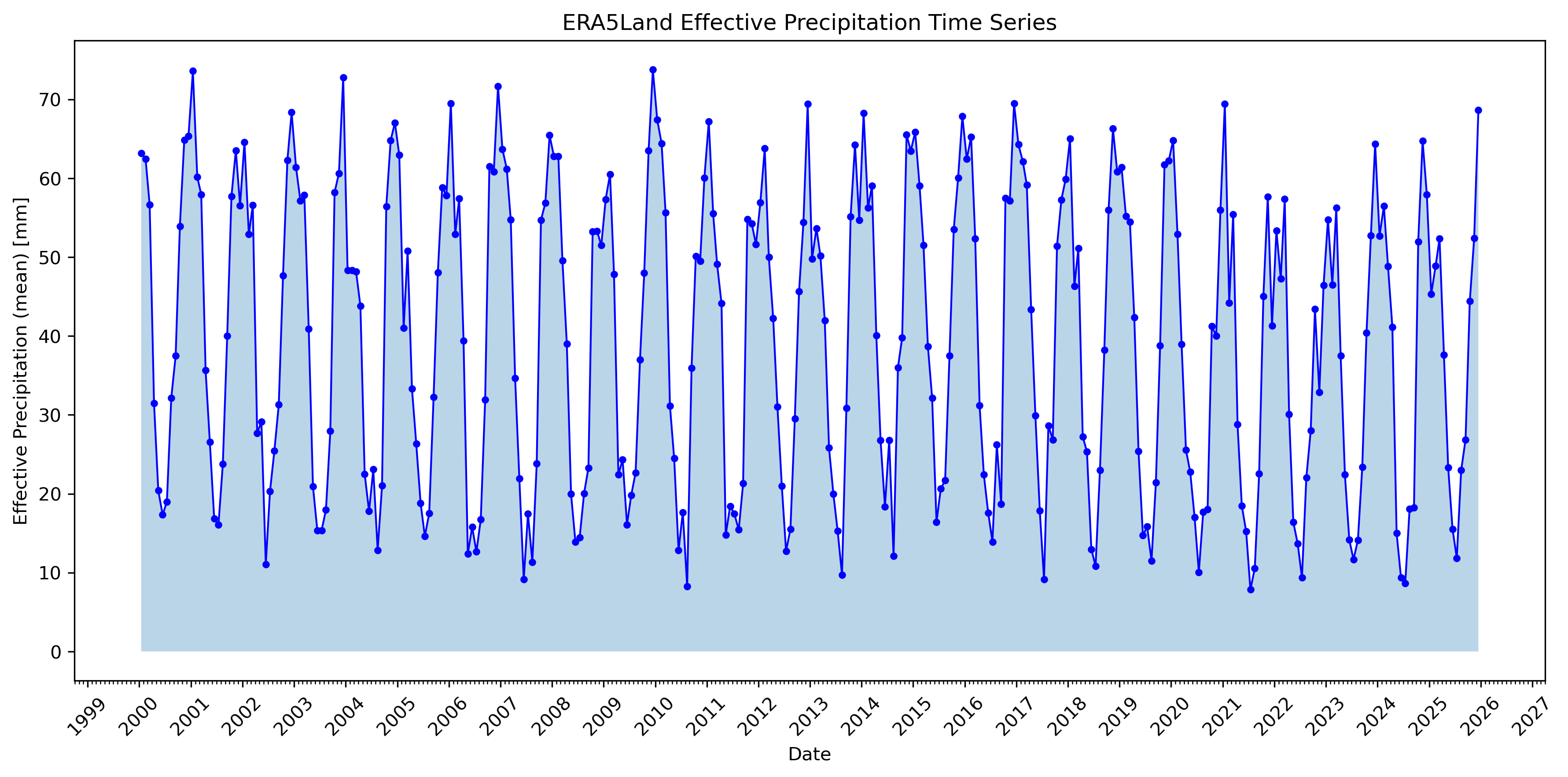
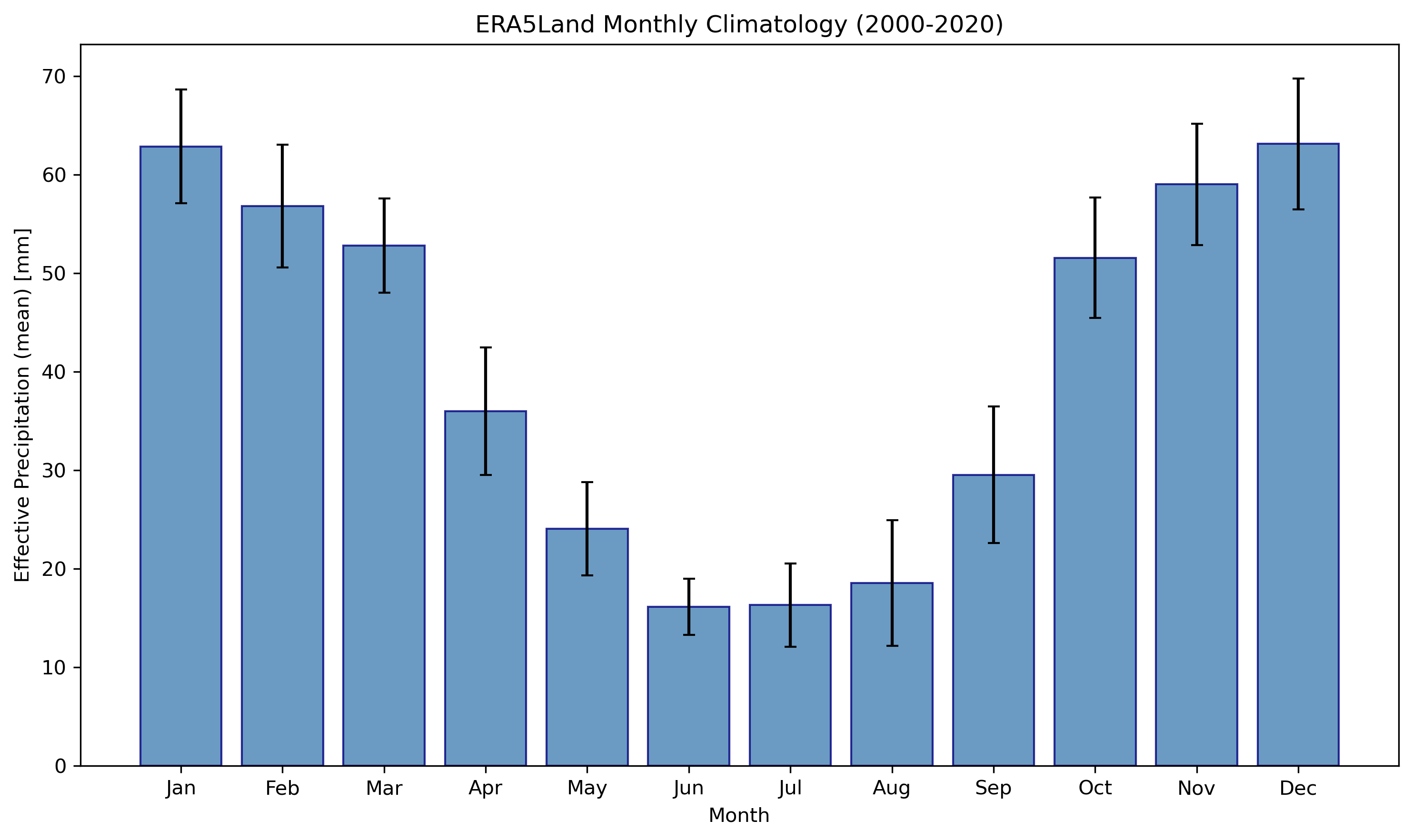
Left: Monthly effective precipitation time series (2000-2025). Right: Monthly climatology showing seasonal patterns.
Spatial Maps
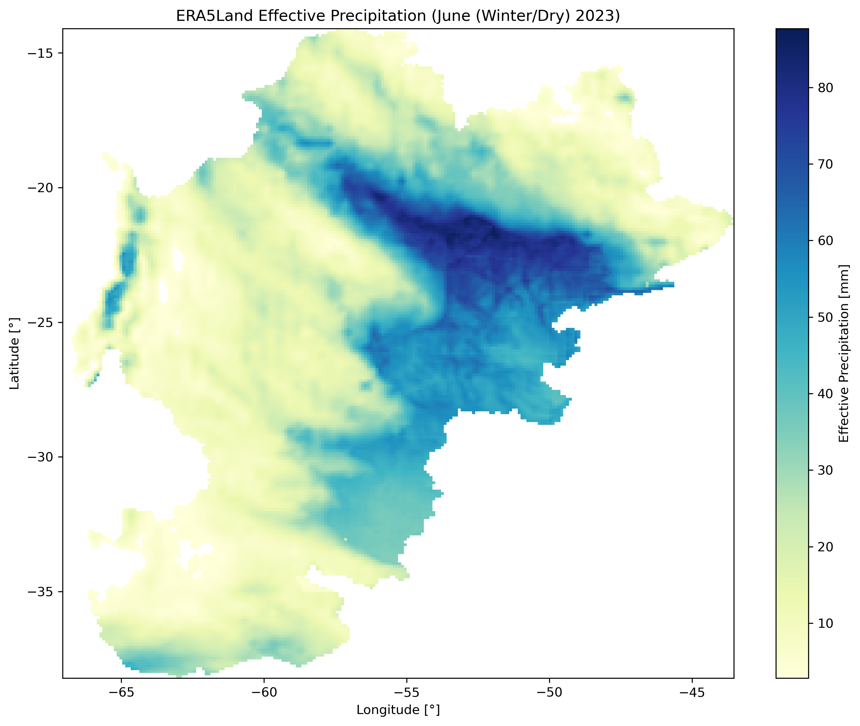
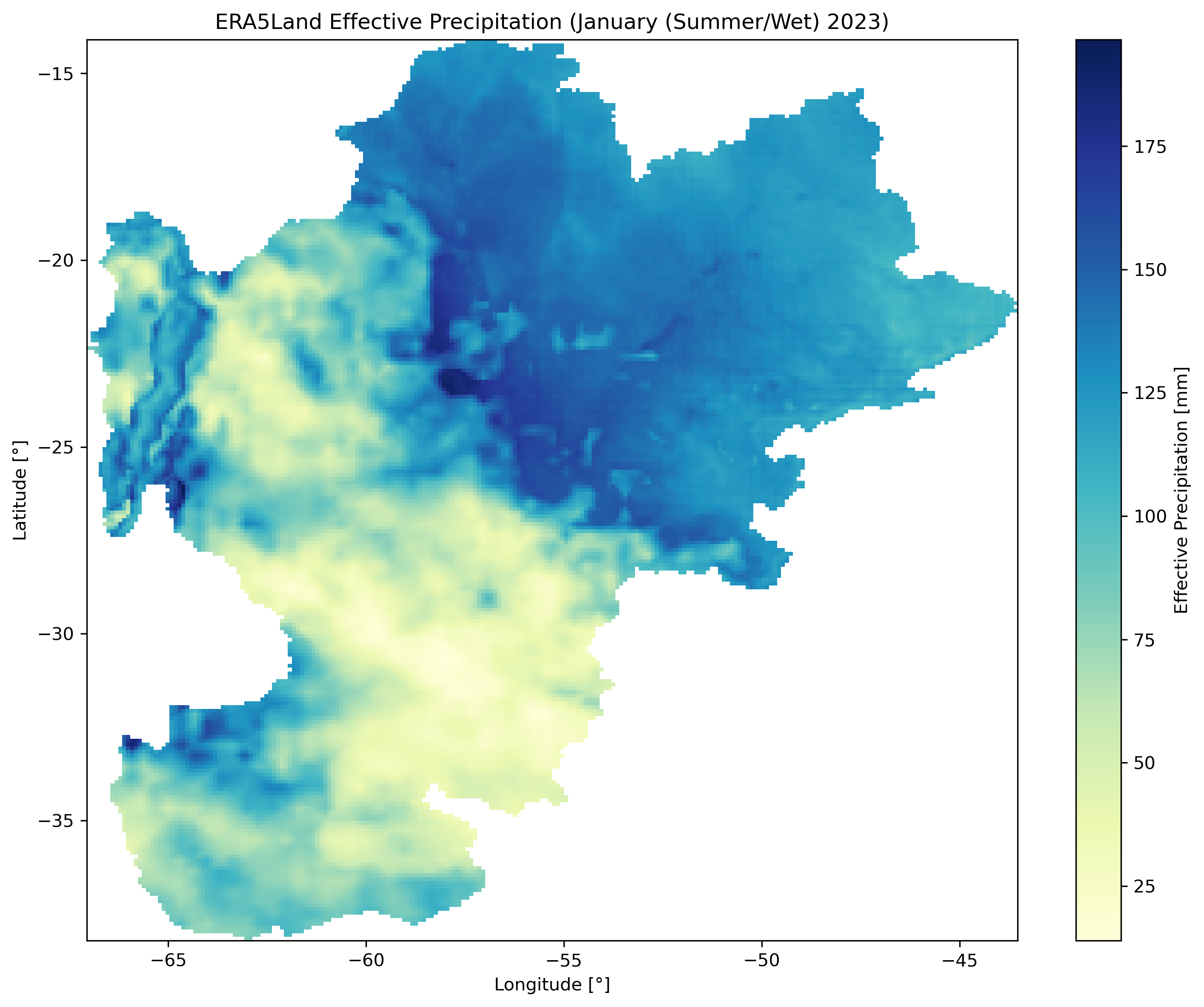
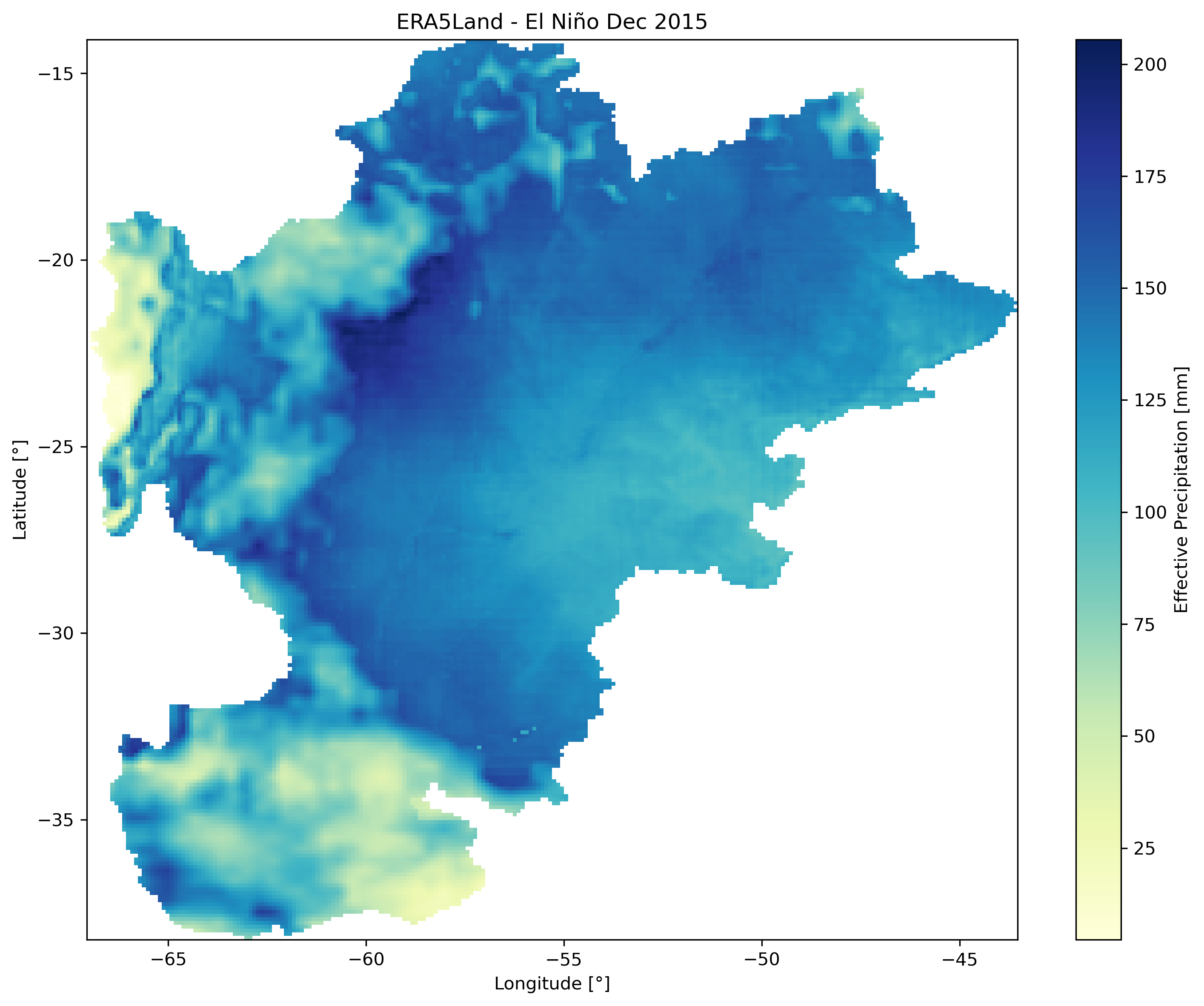
Left: Winter dry season (June 2023). Center: Summer wet season (January 2023). Right: El Niño event (December 2015).
Dataset Comparison (ERA5-Land vs TerraClimate)
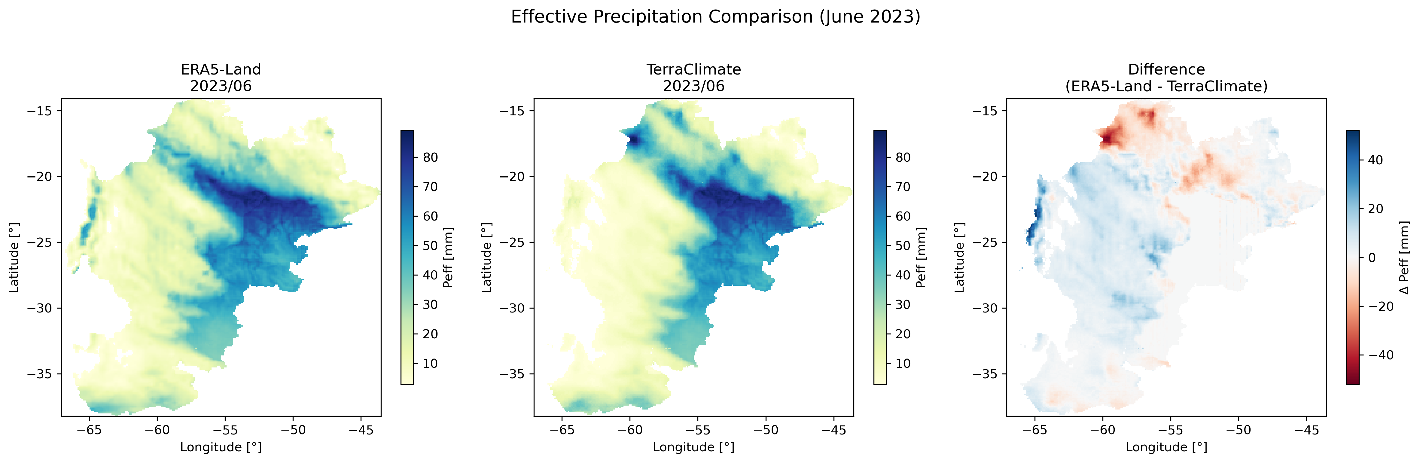
Side-by-side comparison of ERA5-Land and TerraClimate effective precipitation with difference map.
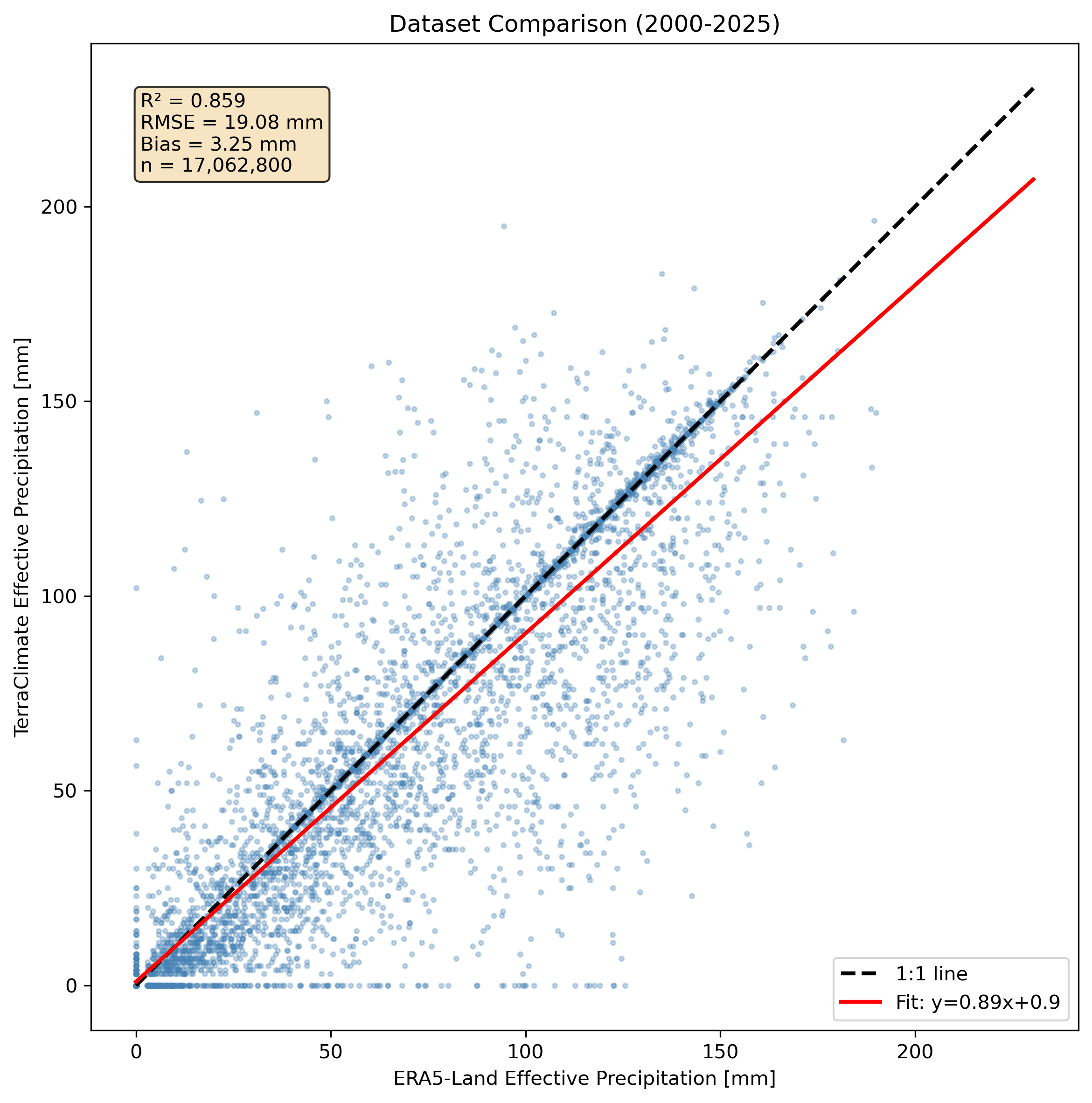
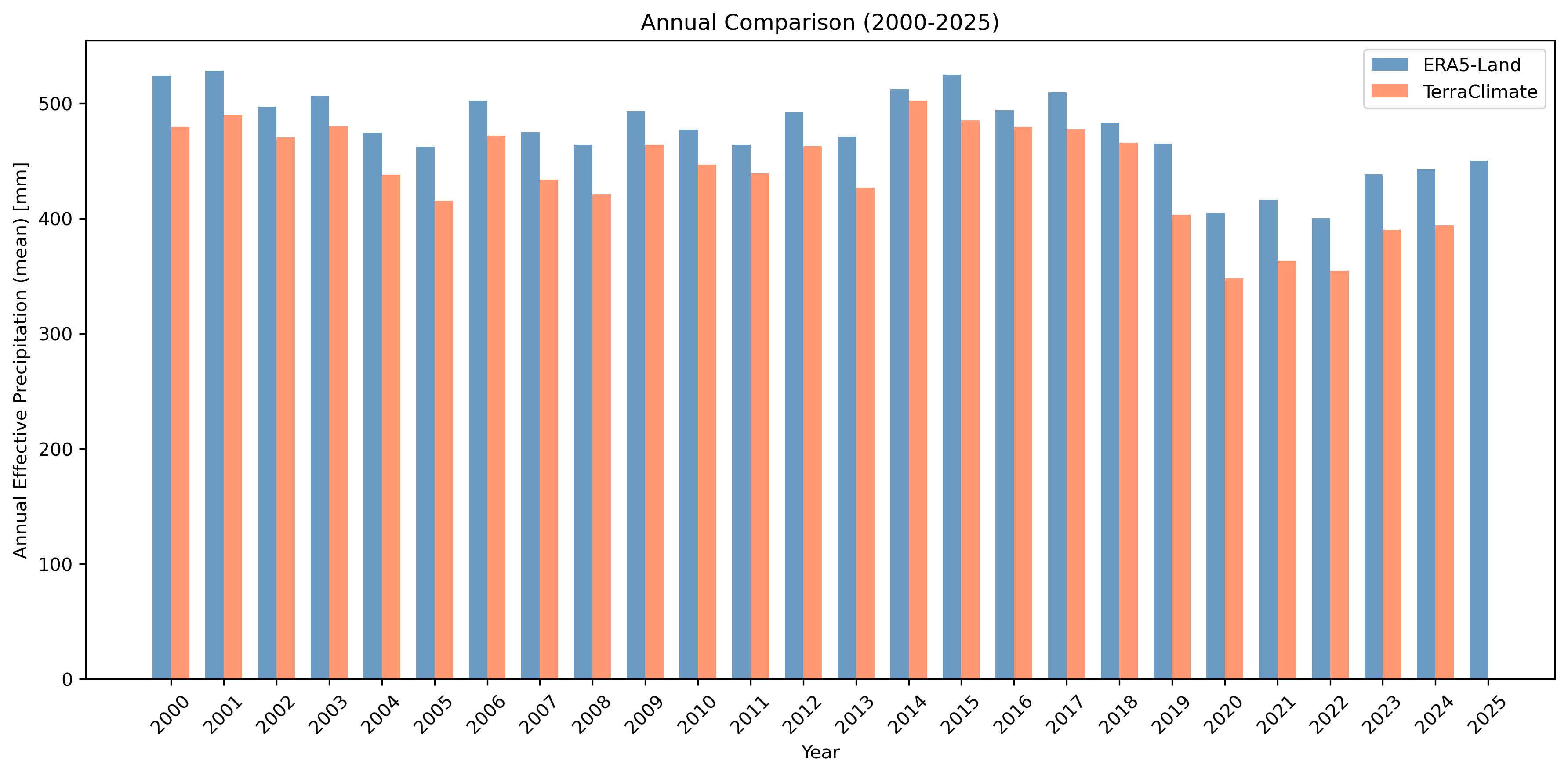
Left: Scatter plot comparison with R², RMSE, and bias statistics. Right: Annual totals comparison.
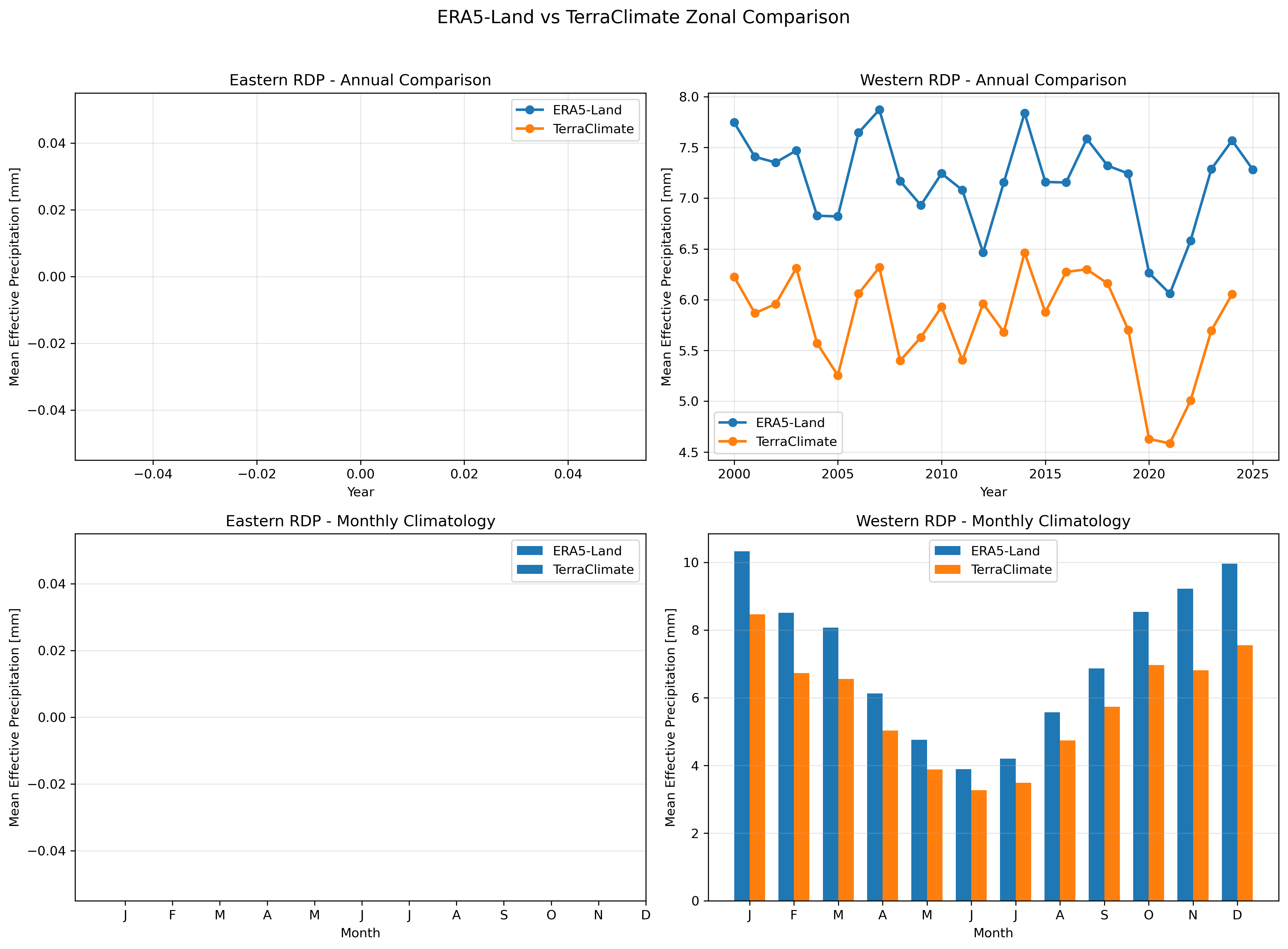
Zonal statistics comparison between ERA5-Land and TerraClimate for Eastern and Western Rio de la Plata regions.
Anomaly, Climatology & Trend Maps
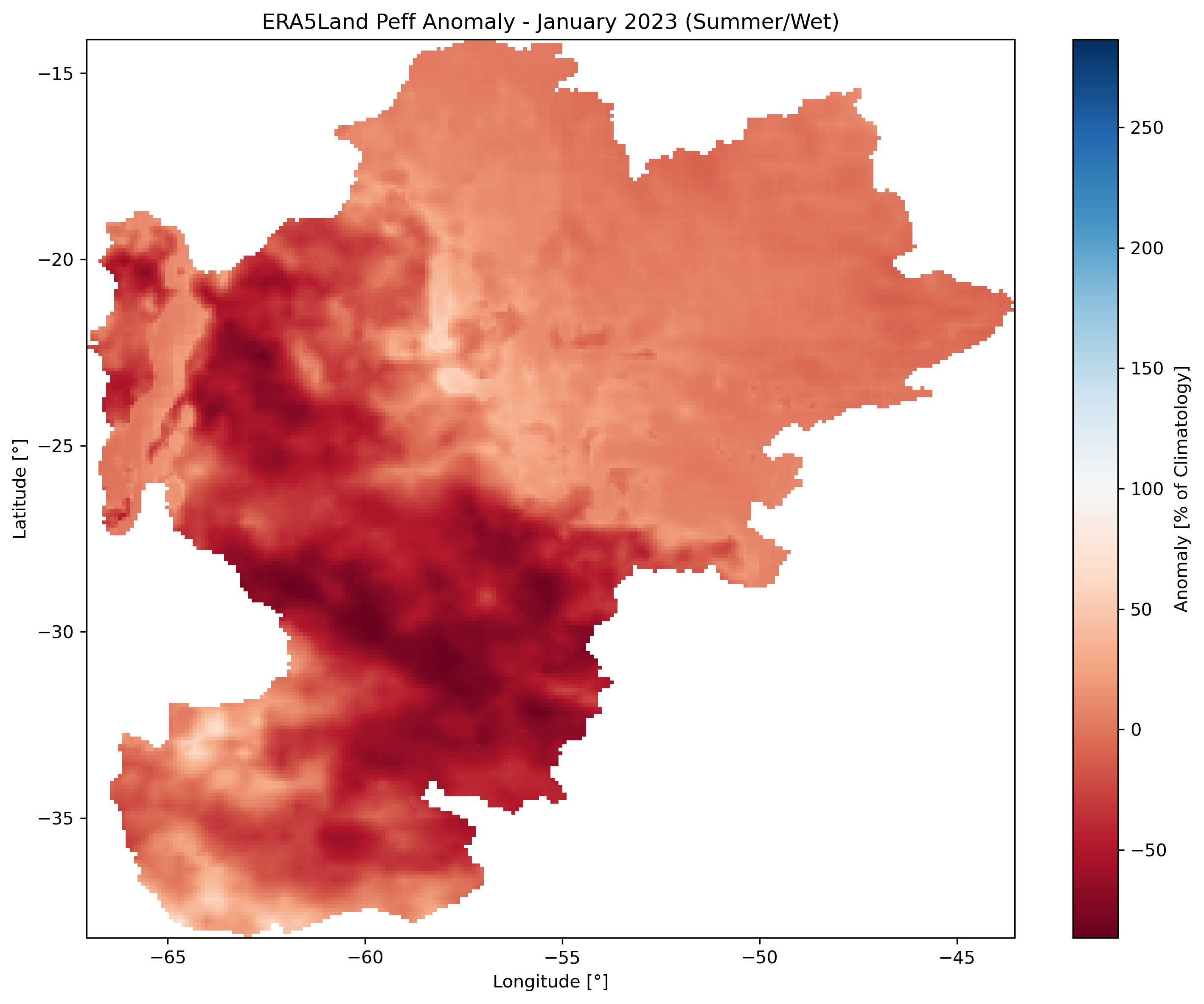
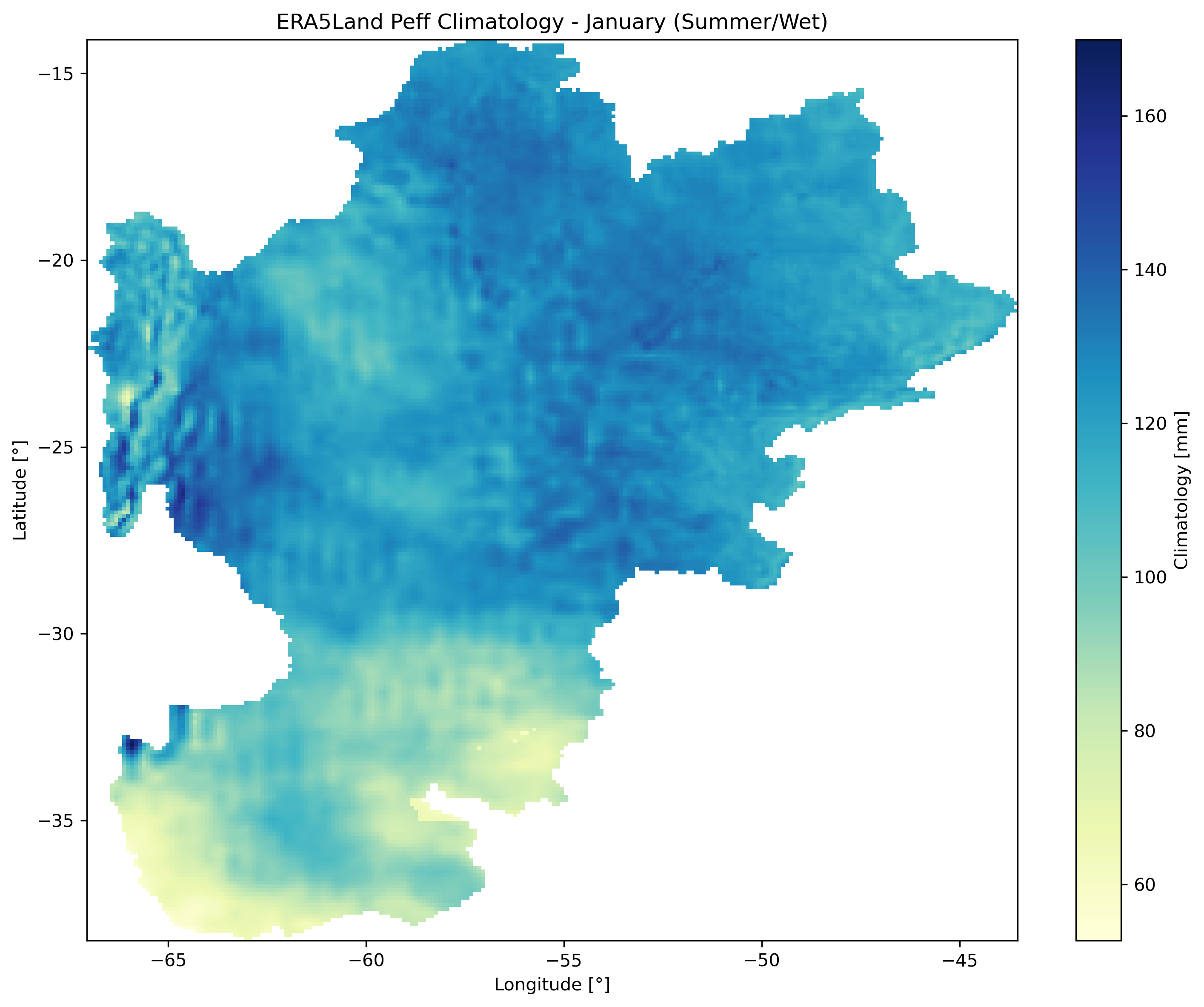
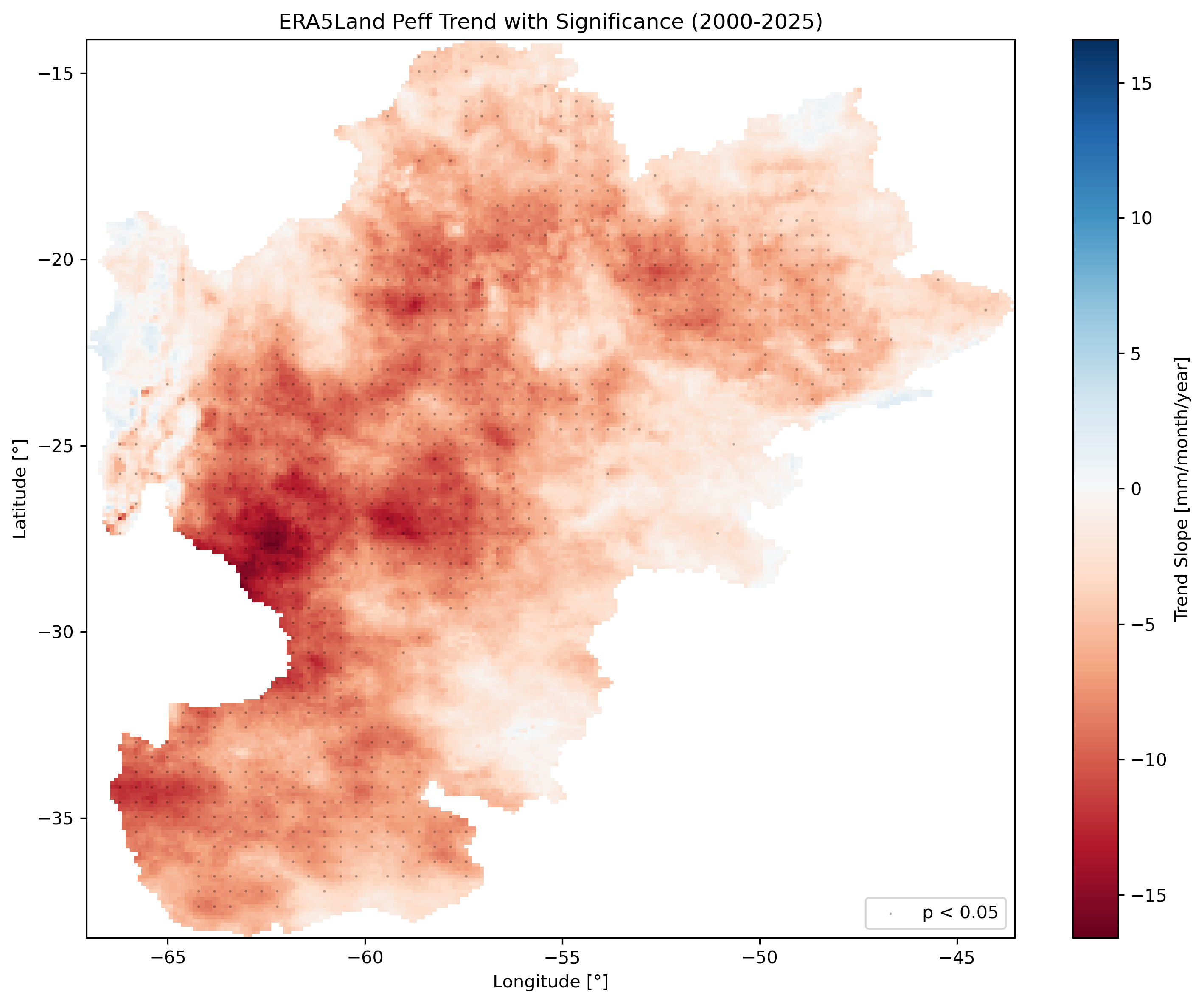
Left: Percent anomaly for January 2023 (diverging colormap centered at 100%). Center: January climatology (2000-2020). Right: Long-term trend with significance stippling (p < 0.05).
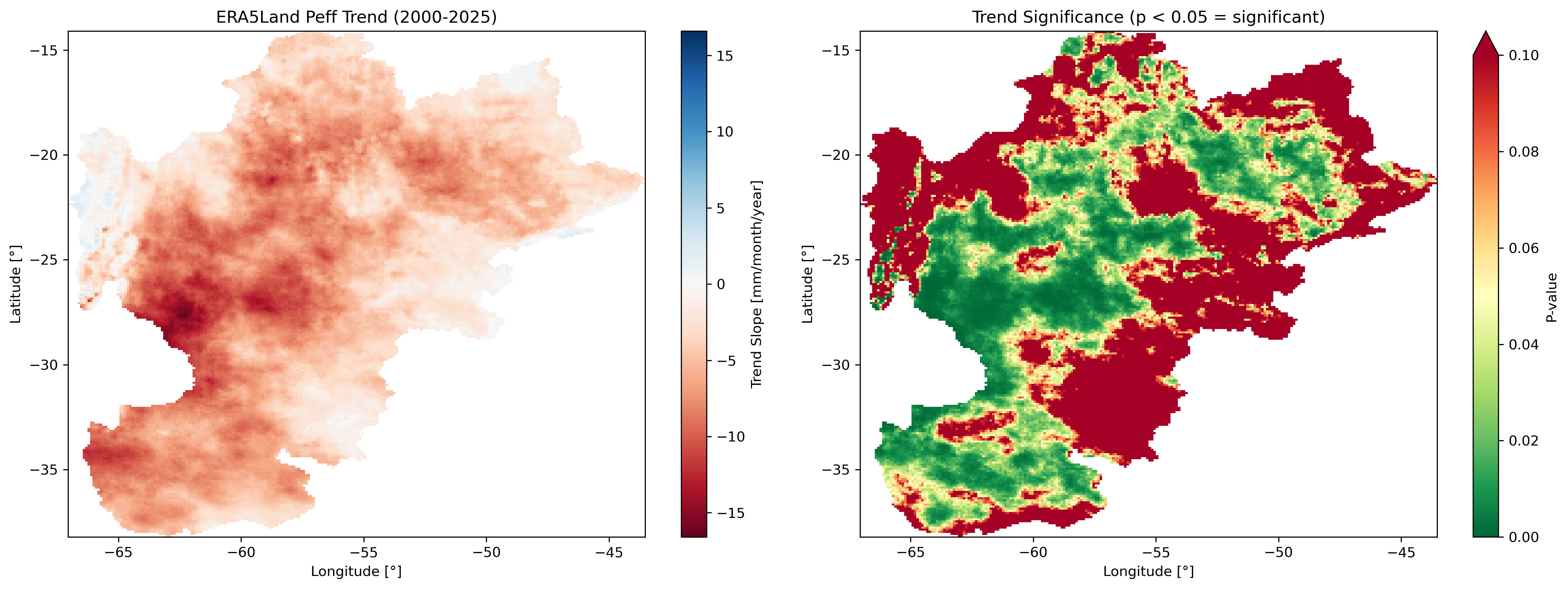
Trend analysis panel showing slope (mm/year) and p-value maps side by side.
Method Comparison
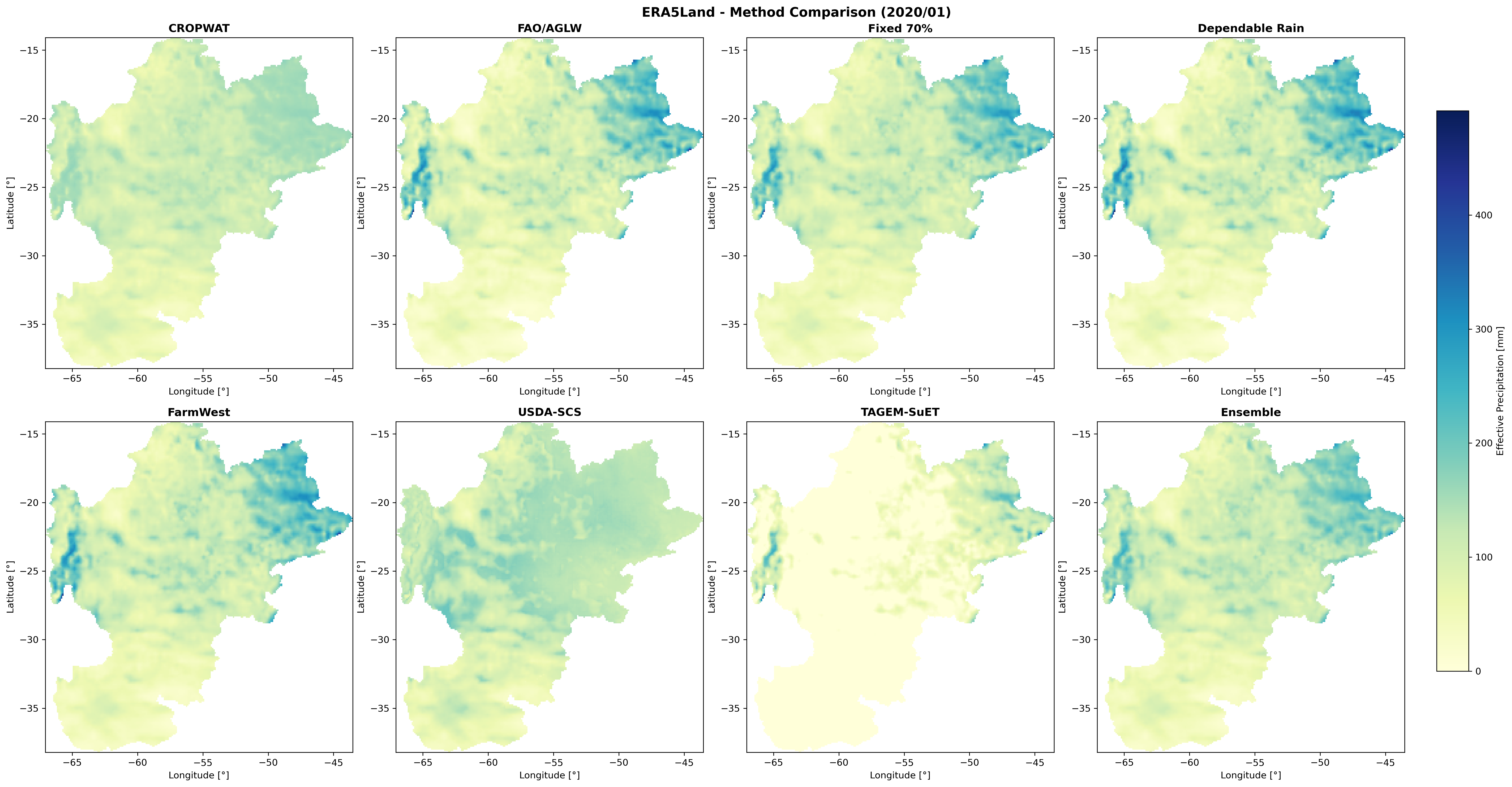
Comparison of effective precipitation methods: CROPWAT, FAO/AGLW, Fixed Percentage (70%), Dependable Rainfall (75%), FarmWest, USDA-SCS, and TAGEM-SuET.
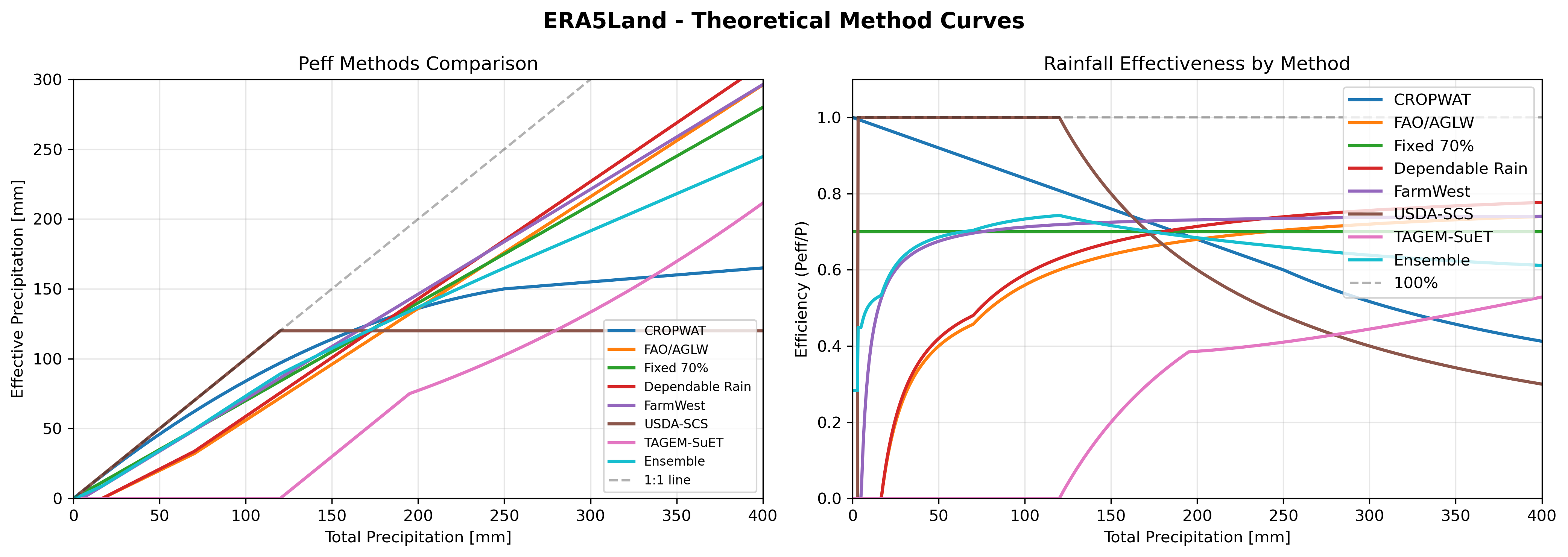
Theoretical response curves for different effective precipitation methods.
Arizona USDA-SCS Example
This example demonstrates the USDA-SCS method for calculating effective precipitation using U.S.-specific datasets for Arizona, with comparisons to global datasets and multiple Peff methods.
Ready-to-Run Script
A comprehensive Arizona workflow is available at Examples/arizona_example.py:
Dataset Configuration
The Arizona example processes 4 precipitation datasets (2 U.S., 2 Global):
| Dataset | Type | GEE Asset ID | Band | Resolution |
|---|---|---|---|---|
| GridMET | U.S. | IDAHO_EPSCOR/GRIDMET |
pr |
~4 km |
| PRISM | U.S. | projects/sat-io/open-datasets/OREGONSTATE/PRISM_800_MONTHLY |
ppt |
~800 m |
| ERA5-Land | Global | ECMWF/ERA5_LAND/MONTHLY_AGGR |
total_precipitation_sum |
~11 km |
| TerraClimate | Global | IDAHO_EPSCOR/TERRACLIMATE |
pr |
~4 km |
For USDA-SCS method, dataset-specific AWC and ETo are used:
U.S. Datasets (High-Resolution):
| Dataset | GEE Asset ID | Description |
|---|---|---|
| AWC (SSURGO) | projects/openet/soil/ssurgo_AWC_WTA_0to152cm_composite |
USDA SSURGO soil water holding capacity |
| ETo (GridMET) | projects/openet/assets/reference_et/conus/gridmet/monthly/v1 |
OpenET GridMET reference ET (band: eto) |
Global Datasets:
| Dataset | GEE Asset ID | Description |
|---|---|---|
| AWC (FAO HWSD) | projects/sat-io/open-datasets/FAO/HWSD_V2_SMU |
FAO Harmonized World Soil Database v2 (band: AWC) |
| ETo (AgERA5) | projects/climate-engine-pro/assets/ce-ag-era5-v2/daily |
AgERA5 FAO-56 Penman-Monteith ETo (band: ReferenceET_PenmanMonteith_FAO56) |
Python Example
from pycropwat import EffectivePrecipitation

# Arizona with GridMET precipitation and USDA-SCS method
ep = EffectivePrecipitation(
    asset_id='IDAHO_EPSCOR/GRIDMET',
    precip_band='pr',
    gee_geometry_asset='users/montimajumdar/AZ',
    start_year=2000,
    end_year=2024,
    scale=4000,  # 4km resolution
    # USDA-SCS specific parameters
    method='usda_scs',
    method_params={
        'awc_asset': 'projects/openet/soil/ssurgo_AWC_WTA_0to152cm_composite',
        'eto_asset': 'projects/openet/assets/reference_et/conus/gridmet/monthly/v1',
        'eto_band': 'eto',
        'rooting_depth': 1.0,  # 1 meter
        'mad_factor': 0.5  # Management Allowed Depletion factor
    }
)

ep.process(output_dir='./Arizona/AZ_GridMET_USDA_SCS', n_workers=8)
CLI Example
# GridMET precipitation with USDA-SCS method for Arizona
pycropwat process --asset IDAHO_EPSCOR/GRIDMET --band pr \
    --gee-geometry users/montimajumdar/AZ \
    --start-year 2000 --end-year 2024 --scale 4000 \
    --method usda_scs \
    --awc-asset projects/openet/soil/ssurgo_AWC_WTA_0to152cm_composite \
    --eto-asset projects/openet/assets/reference_et/conus/gridmet/monthly/v1 \
    --eto-band eto --rooting-depth 1.0 --mad-factor 0.5 \
    --workers 8 --output ./Arizona/AZ_GridMET_USDA_SCS

# PRISM precipitation (higher resolution ~800m)
pycropwat process --asset projects/sat-io/open-datasets/OREGONSTATE/PRISM_800_MONTHLY --band ppt \
    --gee-geometry users/montimajumdar/AZ \
    --start-year 2000 --end-year 2024 --scale 4000 \
    --method usda_scs \
    --awc-asset projects/openet/soil/ssurgo_AWC_WTA_0to152cm_composite \
    --eto-asset projects/openet/assets/reference_et/conus/gridmet/monthly/v1 \
    --eto-band eto --rooting-depth 1.0 --mad-factor 0.5 \
    --workers 8 --output ./Arizona/AZ_PRISM_USDA_SCS
Key Features
- USDA-SCS Method: Accounts for soil water holding capacity (AWC) and evaporative demand (ETo)
- U.S. High-Resolution Data: GridMET (~4km) and PRISM (~800m) precipitation with SSURGO AWC and GridMET ETo
- Global Coverage Data: ERA5-Land and TerraClimate with FAO HWSD AWC and AgERA5 ETo
- ETo Scale Factor: Support for different ETo units via
eto_scale_factorparameter - U.S. vs Global Comparison: Compare U.S. datasets (GridMET, PRISM) against global datasets (ERA5-Land, TerraClimate)
- Method Comparison: Compare all 9 Peff methods (CROPWAT, FAO/AGLW, Fixed %, Dependable Rain, FarmWest, USDA-SCS, TAGEM-SuET, PCML, Ensemble)
- Arizona-Specific Analysis: Monsoon season (Jul-Sep), winter season aggregations
- Regional Zones: Central AZ (Phoenix), Southern AZ (Tucson), Northern AZ (Flagstaff)
Generated Outputs
The workflow generates comprehensive analysis outputs:
Examples/Arizona/
├── AZ_GridMET_USDA_SCS/    # U.S. dataset outputs
├── AZ_PRISM_USDA_SCS/
├── AZ_ERA5Land_USDA_SCS/   # Global dataset outputs
├── AZ_TerraClimate_USDA_SCS/
└── analysis_outputs/
    ├── annual/             # Temporal aggregations
    ├── climatology/
    ├── anomalies/          # Statistical analysis & CSV exports
    ├── trend/
    ├── figures/            # Raster maps & time series plots
    ├── comparisons/
    ├── zonal_stats/
    ├── us_vs_global/       # U.S. vs Global dataset comparison
    │   ├── us_global_spatial_*.png
    │   ├── multi_dataset_summary.png
    │   └── dataset_statistics.csv
    ├── method_comparison/  # All 8 methods comparison
    │   ├── method_spatial_*.png
    │   ├── method_curves_arizona.png
    │   ├── method_comparison_summary.png
    │   └── method_statistics.csv
    ├── az_zones.geojson
    └── *_usda_scs_peff_2000_2024.nc
Arizona Example Outputs
The Arizona workflow generates the following visualizations:
Time Series & Climatology
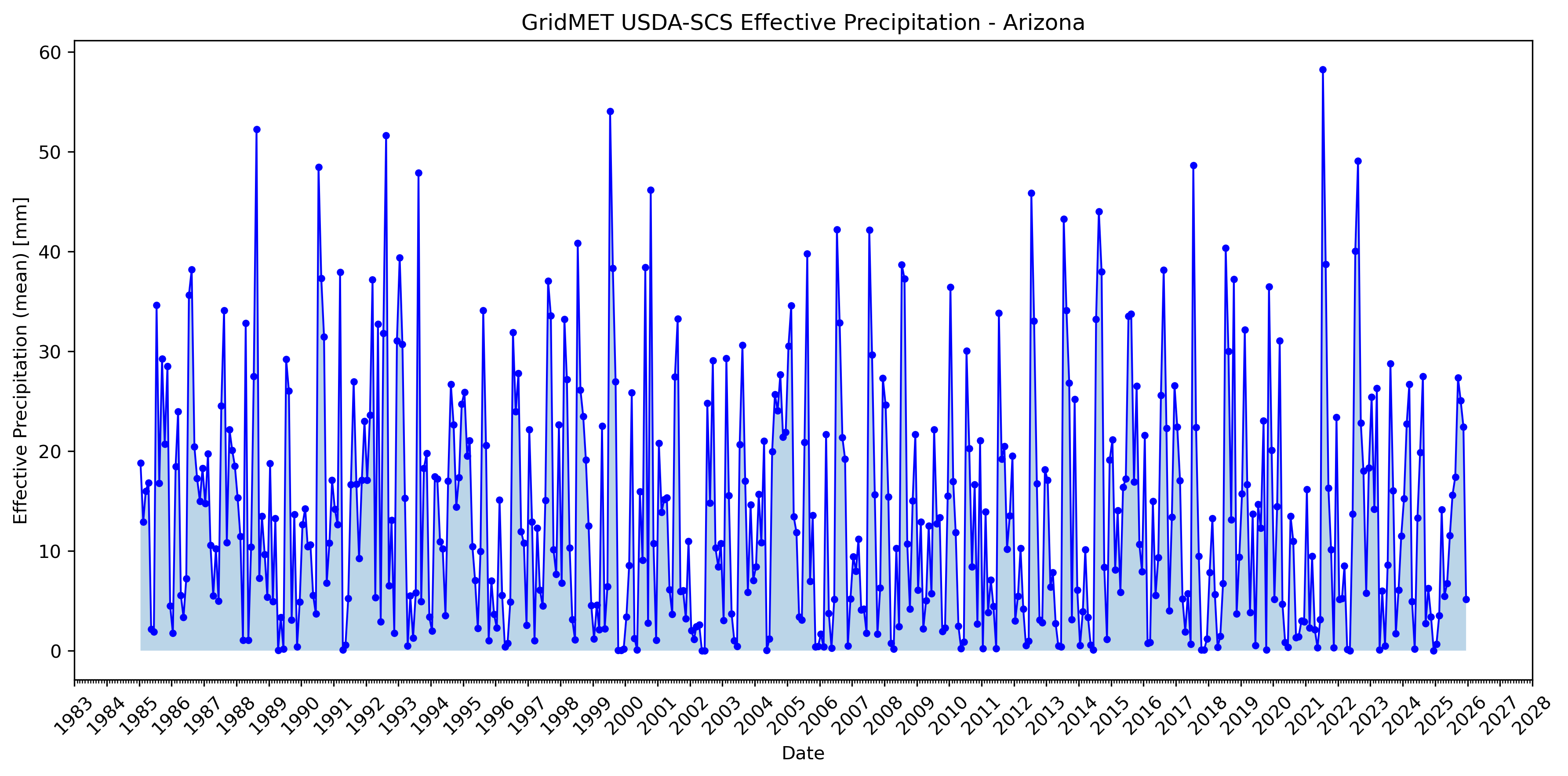
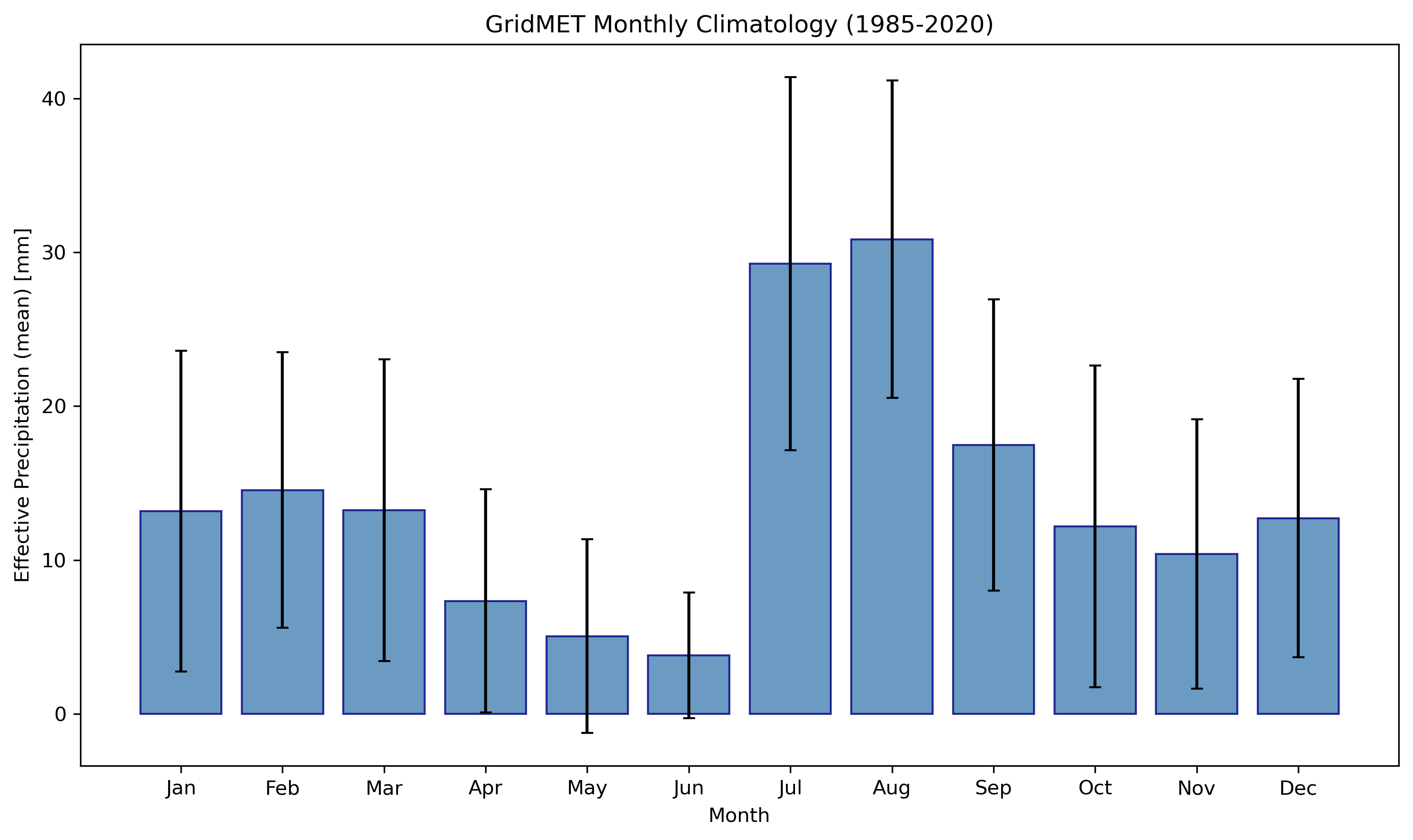
GridMET USDA-SCS effective precipitation for Arizona: time series (left) and monthly climatology (right).
Anomaly, Climatology & Trend Maps
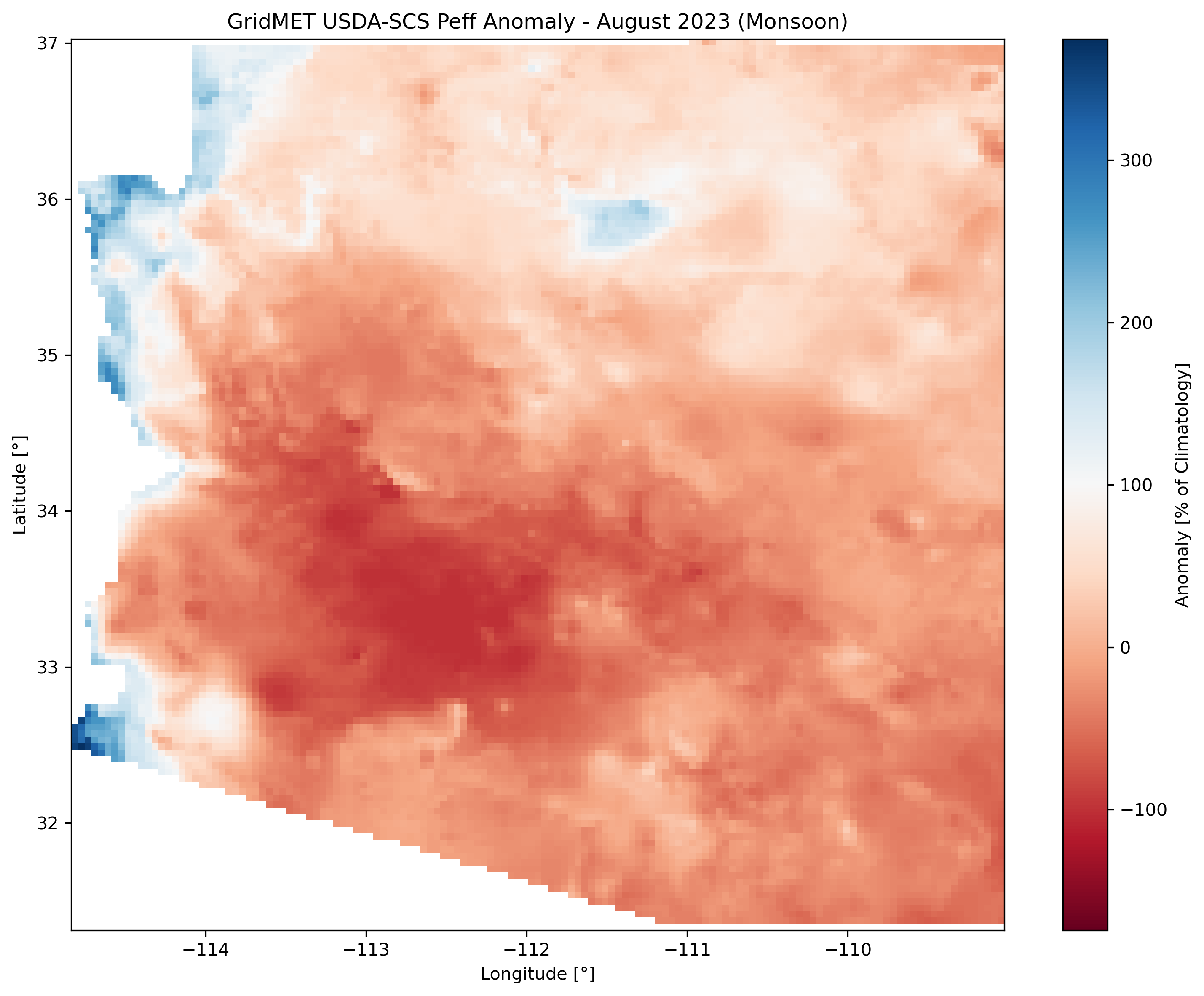
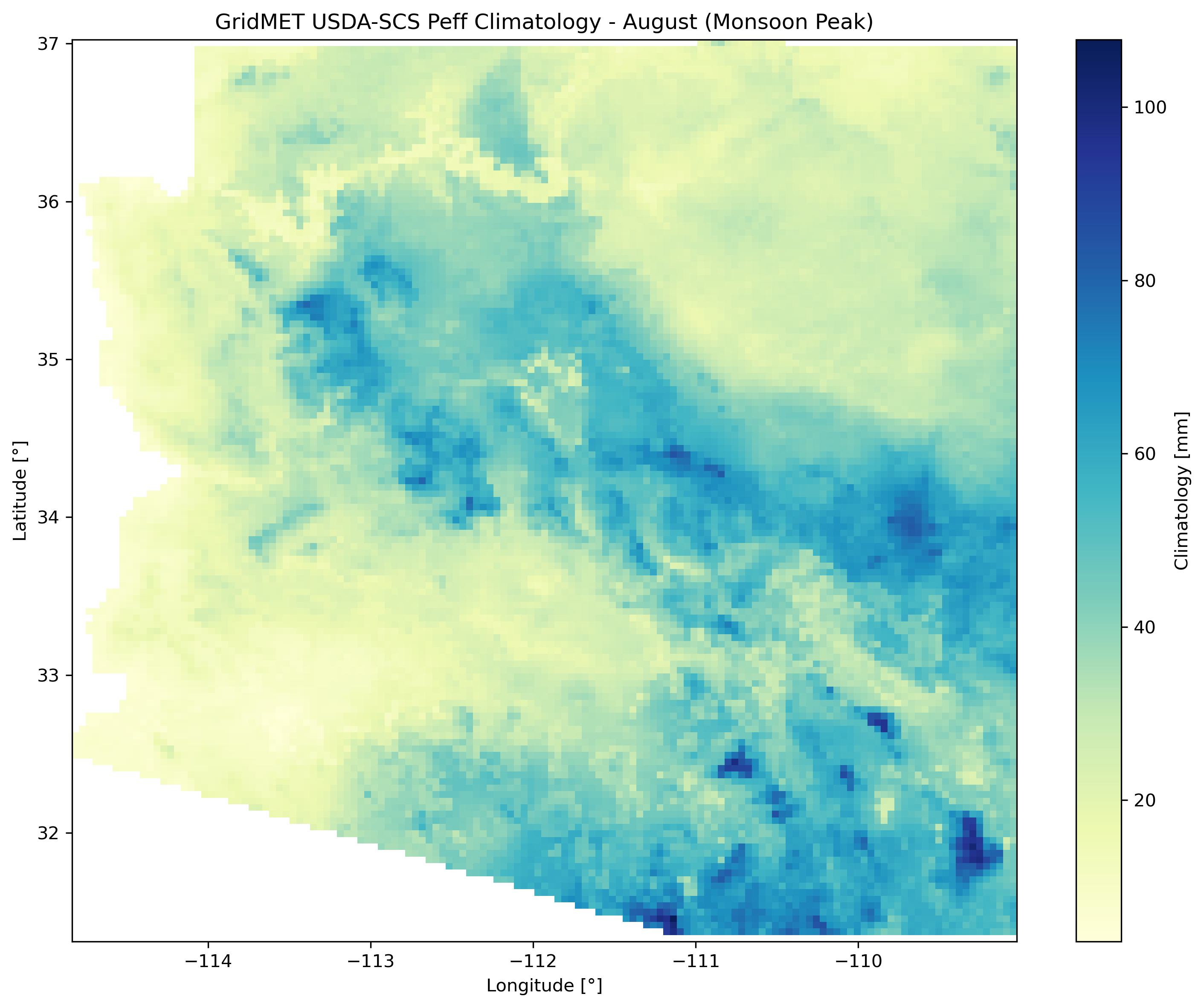
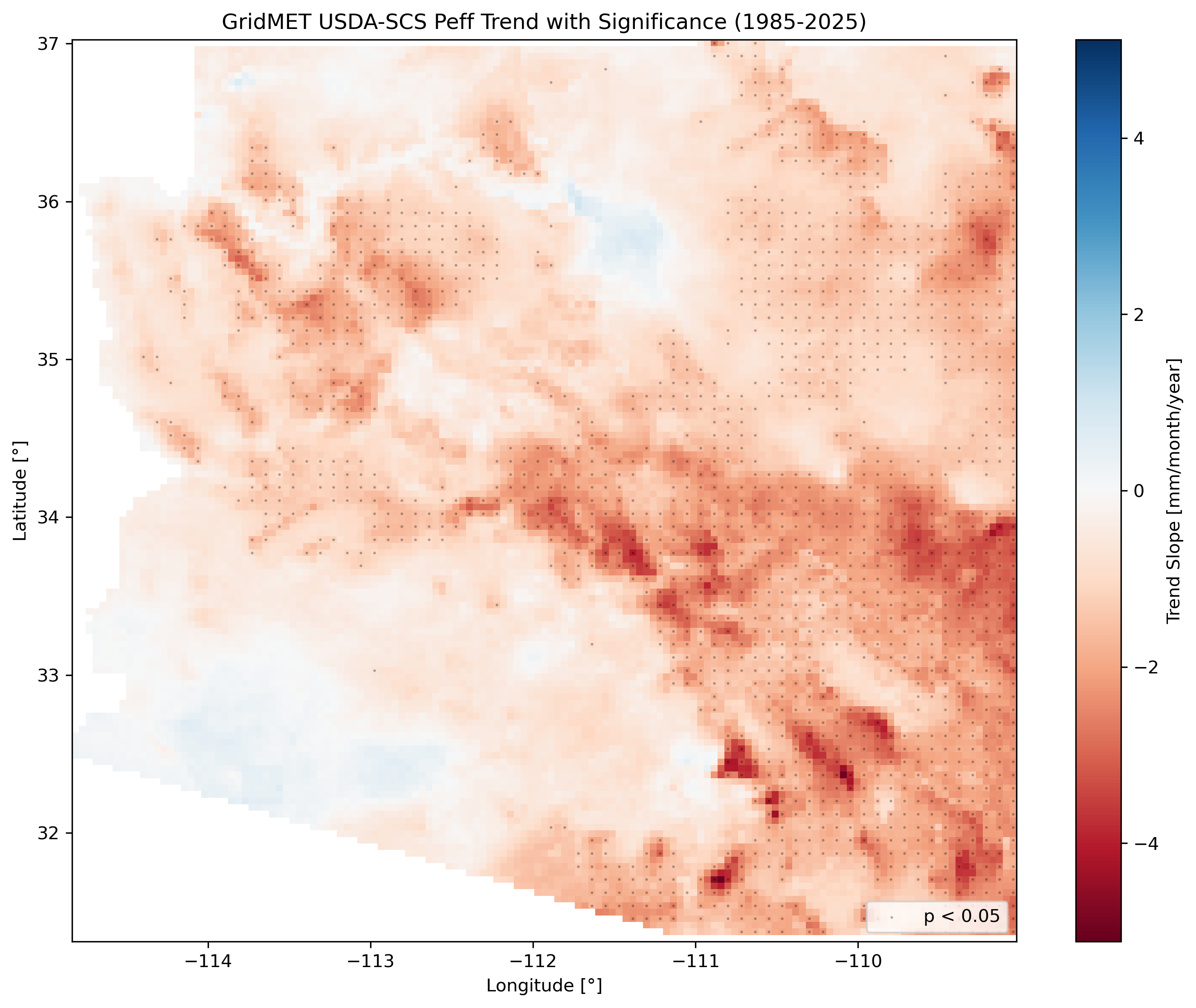
Left: August 2023 anomaly (monsoon season). Center: August climatology (monsoon peak). Right: Long-term trend with significance stippling (p < 0.05).
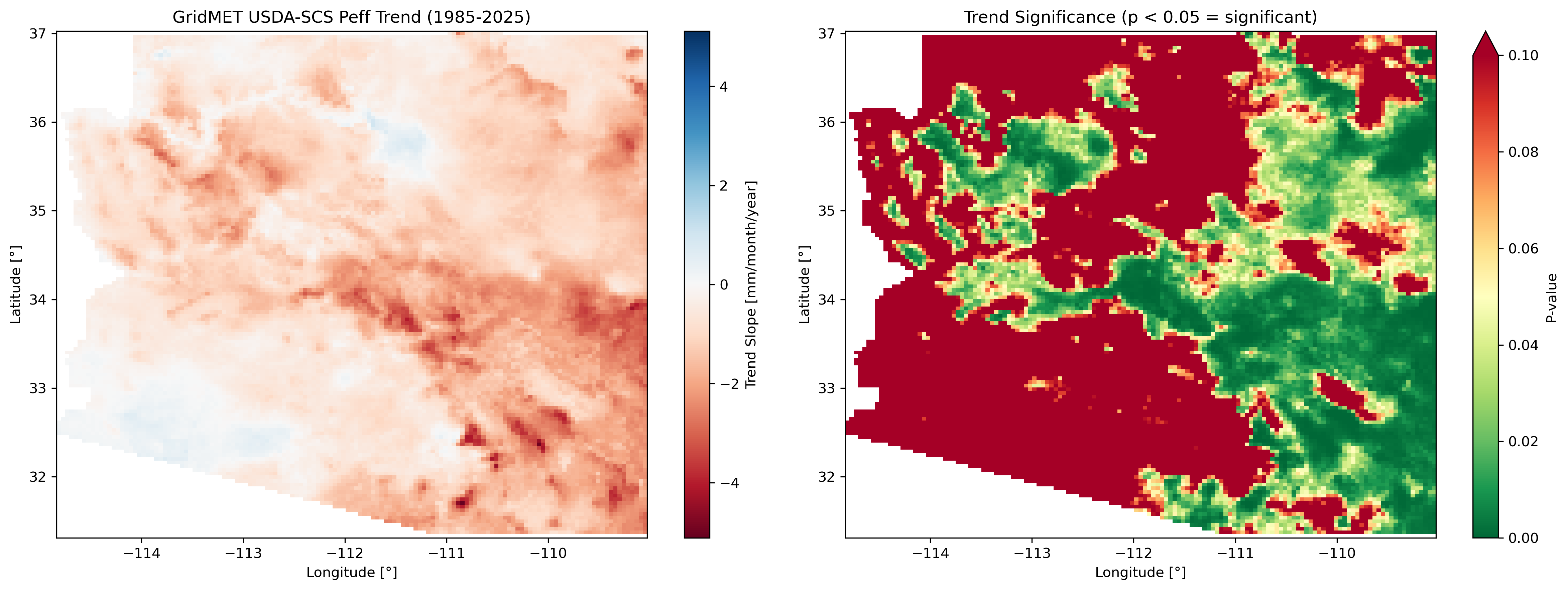
Trend analysis panel for Arizona showing slope (mm/year) and p-value maps side by side.
U.S. vs Global Dataset Comparison
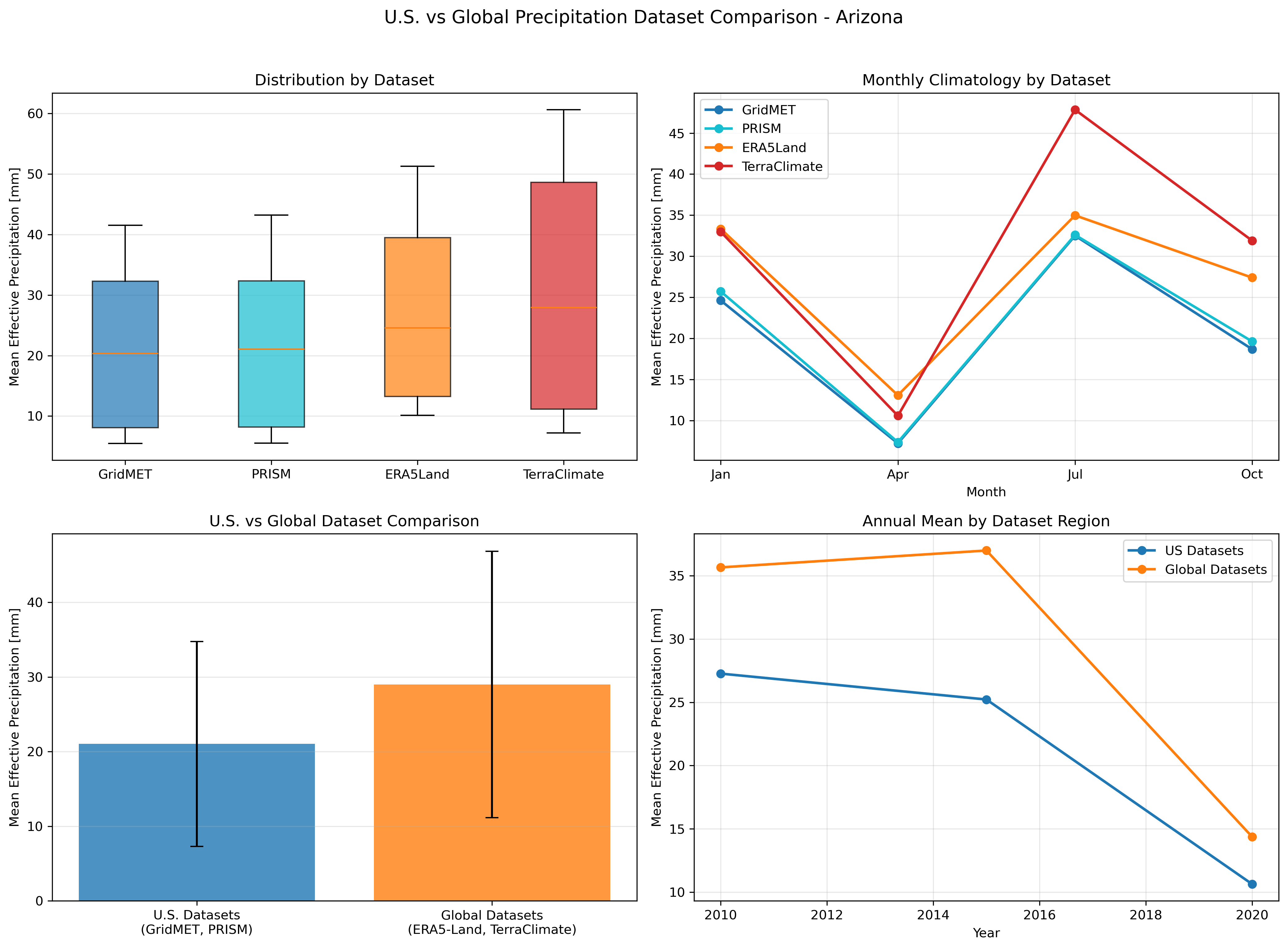
Comparison of U.S. datasets (GridMET, PRISM) vs Global datasets (ERA5-Land, TerraClimate) for Arizona.
Method Comparison
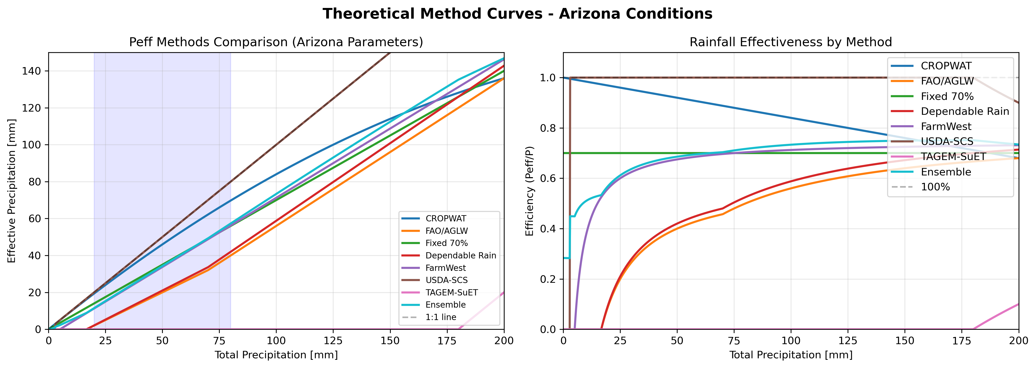
Theoretical Peff response curves for Arizona conditions (AWC=150 mm/m, ETo=180 mm/month).
New Mexico Method Comparison Example
This example demonstrates an efficient workflow for comparing 8 effective precipitation methods across New Mexico using high-resolution PRISM precipitation data (~800m). The workflow downloads rasters once using USDA-SCS, then calculates all other methods locally. Note: PCML is excluded since this workflow uses local method calculations rather than GEE asset downloads.
Ready-to-Run Script
A comprehensive New Mexico workflow is available at Examples/new_mexico_example.py:
Efficient Workflow Design
The New Mexico example uses a single-download approach for efficiency:
- Download once: Use USDA-SCS method to download P (PRISM), AWC (SSURGO), and ETo (gridMET) rasters
- Calculate locally: Load saved rasters and calculate all 9 Peff methods using
pycropwat.methods - Analyze: Perform temporal aggregation, statistical analysis, and export to NetCDF
- Visualize: Create method comparison maps, curves, and statistics
Dataset Configuration
| Component | GEE Asset ID | Band | Resolution |
|---|---|---|---|
| Precipitation | projects/sat-io/open-datasets/OREGONSTATE/PRISM_800_MONTHLY |
ppt |
~800 m |
| AWC (SSURGO) | projects/openet/soil/ssurgo_AWC_WTA_0to152cm_composite |
- | ~30 m |
| ETo (gridMET) | projects/openet/assets/reference_et/conus/gridmet/monthly/v1 |
eto |
~4 km |
Python Example
from pycropwat import EffectivePrecipitation
from pycropwat.methods import (
    cropwat_effective_precip,
    fao_aglw_effective_precip,
    fixed_percentage_effective_precip,
    dependable_rainfall_effective_precip,
    farmwest_effective_precip,
    usda_scs_effective_precip,
    suet_effective_precip,
    ensemble_effective_precip
)
import rioxarray
import numpy as np

# Step 1: Download rasters using USDA-SCS method
ep = EffectivePrecipitation(
    asset_id='projects/sat-io/open-datasets/OREGONSTATE/PRISM_800_MONTHLY',
    precip_band='ppt',
    geometry_path='NM.geojson',
    start_year=1986,
    end_year=2025,
    scale=800,
    method='usda_scs',
    method_params={
        'awc_asset': 'projects/openet/soil/ssurgo_AWC_WTA_0to152cm_composite',
        'eto_asset': 'projects/openet/assets/reference_et/conus/gridmet/monthly/v1',
        'eto_band': 'eto'
    }
)
ep.process(output_dir='./NewMexico/NM_PRISM_USDA_SCS', n_workers=4)

# Step 2: Calculate all methods from saved rasters
precip = rioxarray.open_rasterio('precip_2020_08.tif').squeeze().values
awc = rioxarray.open_rasterio('awc.tif').squeeze().values
eto = rioxarray.open_rasterio('eto_2020_08.tif').squeeze().values

# Calculate all 8 methods
methods = {
    'cropwat': cropwat_effective_precip(precip),
    'fao_aglw': fao_aglw_effective_precip(precip),
    'fixed_percentage': fixed_percentage_effective_precip(precip, 0.7),
    'dependable_rainfall': dependable_rainfall_effective_precip(precip, 0.75),
    'farmwest': farmwest_effective_precip(precip),
    'usda_scs': usda_scs_effective_precip(precip, eto, awc),
    'suet': suet_effective_precip(precip, eto),
    'ensemble': ensemble_effective_precip(precip, eto, awc)
}
Key Features
- Efficient Single-Download: Download P, AWC, ETo once with USDA-SCS, then calculate all methods locally
- All 9 Peff Methods: CROPWAT, FAO/AGLW, Fixed %, Dependable Rain, FarmWest, USDA-SCS, TAGEM-SuET, PCML, Ensemble
- High-Resolution PRISM: ~800m precipitation data for detailed spatial analysis
- U.S. Soil & Climate Data: SSURGO AWC and gridMET ETo
- Long-term Analysis: 1986-2025 (40 years) for trend detection
- New Mexico Specific: Monsoon season (Jul-Sep) and winter season (Nov-Mar) aggregations
- Regional Zones: Northern, Central, Southern, and Eastern New Mexico
Generated Outputs
Examples/NewMexico/
├── NM_PRISM_USDA_SCS/          # Downloaded rasters (P, AWC, ETo)
│   ├── awc.tif
│   ├── eto_{year}_{month}.tif
│   ├── effective_precip_{year}_{month}.tif
│   └── effective_precip_fraction_{year}_{month}.tif
└── analysis_outputs/
    ├── peff_by_method/         # Calculated Peff for each method
    │   ├── cropwat/
    │   ├── fao_aglw/
    │   ├── fixed_percentage/
    │   ├── dependable_rainfall/
    │   ├── farmwest/
    │   ├── usda_scs/
    │   └── suet/
    ├── annual/                  # Temporal aggregations by method
    ├── climatology/
    ├── anomalies/
    ├── trend/
    ├── monsoon_season/
    ├── winter_season/
    ├── method_comparison/       # All 8 methods comparison
        ├── method_maps_*.png
    │   ├── method_curves_new_mexico.png
    │   ├── mean_annual_comparison_*.png
    │   └── method_statistics.csv
    ├── nm_zones.geojson
    └── NM_PRISM_*_peff_1986_2025.nc
Example 13: Drought Monitoring Dashboard
Build a drought monitoring system using effective precipitation anomalies.
Python:
from pycropwat import EffectivePrecipitation
from pycropwat.analysis import TemporalAggregator, StatisticalAnalyzer, Visualizer
import pandas as pd
from pathlib import Path
from datetime import datetime

class DroughtMonitor:
    """Simple drought monitoring using Peff anomalies."""

    def __init__(self, output_dir: str):
        self.output_dir = Path(output_dir)
        self.agg = TemporalAggregator(output_dir)
        self.stats = StatisticalAnalyzer(output_dir)
        self.viz = Visualizer(output_dir)

    def calculate_drought_index(self, year: int, month: int,
                                 clim_start: int = 1990, clim_end: int = 2020):
        """Calculate standardized drought index (SPI-like for Peff)."""
        anomaly = self.stats.calculate_anomaly(
            year=year, month=month,
            clim_start=clim_start, clim_end=clim_end,
            anomaly_type='standardized'  # z-score
        )
        return anomaly

    def classify_drought(self, z_score):
        """Classify drought based on standardized anomaly."""
        # SPI-like classification
        if z_score >= 2.0:
            return "Extremely Wet"
        elif z_score >= 1.5:
            return "Very Wet"
        elif z_score >= 1.0:
            return "Moderately Wet"
        elif z_score > -1.0:
            return "Near Normal"
        elif z_score > -1.5:
            return "Moderate Drought"
        elif z_score > -2.0:
            return "Severe Drought"
        else:
            return "Extreme Drought"

    def generate_monthly_report(self, year: int, month: int):
        """Generate monthly drought monitoring report."""
        import numpy as np

        # Calculate anomaly
        anomaly = self.calculate_drought_index(year, month)

        # Get spatial statistics
        mean_z = float(anomaly.mean())
        min_z = float(anomaly.min())
        max_z = float(anomaly.max())

        # Calculate percent area in drought
        drought_mask = anomaly < -1.0
        drought_pct = float(drought_mask.sum() / drought_mask.size * 100)

        # Generate report
        report = {
            'date': f"{year}-{month:02d}",
            'mean_anomaly': mean_z,
            'min_anomaly': min_z,
            'max_anomaly': max_z,
            'drought_classification': self.classify_drought(mean_z),
            'percent_area_drought': drought_pct
        }

        # Create visualization
        self.viz.plot_anomaly_map(
            anomaly_path=f'./anomalies/anomaly_{year}_{month:02d}.tif',
            title=f'Drought Index - {year}/{month:02d}\n{self.classify_drought(mean_z)}',
            output_path=f'./reports/drought_{year}_{month:02d}.png'
        )

        return report

# Usage
monitor = DroughtMonitor('./outputs')

# Generate reports for 2023
reports = []
for month in range(1, 13):
    report = monitor.generate_monthly_report(2023, month)
    reports.append(report)
    print(f"{report['date']}: {report['drought_classification']} "
          f"({report['percent_area_drought']:.1f}% in drought)")

# Save summary
pd.DataFrame(reports).to_csv('./reports/drought_summary_2023.csv', index=False)
Example 14: Irrigation Scheduling Support
Calculate crop water requirements using effective precipitation.
Python:
from pycropwat import EffectivePrecipitation
from pycropwat.analysis import TemporalAggregator
import numpy as np
import xarray as xr
import rioxarray

def calculate_irrigation_requirement(
    peff_path: str,
    etc_path: str,  # Crop ET path
    output_path: str
) -> xr.DataArray:
    """
    Calculate net irrigation requirement.

    NIR = ETc - Peff (where ETc > Peff)
    """
    peff = rioxarray.open_rasterio(peff_path).squeeze('band', drop=True)
    etc = rioxarray.open_rasterio(etc_path).squeeze('band', drop=True)

    # Net irrigation requirement
    nir = np.maximum(etc - peff, 0)

    nir.attrs = {
        'units': 'mm',
        'long_name': 'net_irrigation_requirement'
    }
    nir.rio.to_raster(output_path)

    return nir


def monthly_irrigation_schedule(
    peff_dir: str,
    etc_values: dict,  # {month: etc_mm}
    year: int
) -> dict:
    """
    Generate monthly irrigation schedule for a crop.

    Parameters
    ----------
    peff_dir : str
        Directory with effective precipitation rasters
    etc_values : dict
        Monthly crop ET values in mm (e.g., from FAO-56)
    year : int
        Year to analyze

    Returns
    -------
    dict
        Monthly irrigation requirements
    """
    agg = TemporalAggregator(peff_dir)
    schedule = {}

    for month, etc in etc_values.items():
        # Get monthly Peff
        if year in agg._index and month in agg._index[year]:
            peff_da = rioxarray.open_rasterio(
                agg._index[year][month]
            ).squeeze('band', drop=True)

            mean_peff = float(peff_da.mean())
            nir = max(etc - mean_peff, 0)

            schedule[month] = {
                'etc_mm': etc,
                'peff_mm': mean_peff,
                'nir_mm': nir,
                'peff_fraction': mean_peff / etc if etc > 0 else 0
            }

    return schedule


# Example: Maize irrigation schedule for Arizona
# ETc values from FAO-56 for maize (April-October growing season)
maize_etc = {
    4: 75,   # April - initial stage
    5: 120,  # May - development
    6: 180,  # June - mid-season
    7: 200,  # July - mid-season (peak)
    8: 180,  # August - mid-season
    9: 120,  # September - late season
    10: 60   # October - harvest
}

schedule = monthly_irrigation_schedule(
    peff_dir='./Arizona/AZ_GridMET_USDA_SCS',
    etc_values=maize_etc,
    year=2023
)

print("\nMaize Irrigation Schedule - Arizona 2023")
print("-" * 60)
print(f"{'Month':<10} {'ETc':>8} {'Peff':>8} {'NIR':>8} {'Peff%':>8}")
print("-" * 60)

total_etc = 0
total_peff = 0
total_nir = 0

for month, data in schedule.items():
    month_name = ['Jan','Feb','Mar','Apr','May','Jun',
                  'Jul','Aug','Sep','Oct','Nov','Dec'][month-1]
    print(f"{month_name:<10} {data['etc_mm']:>8.1f} {data['peff_mm']:>8.1f} "
          f"{data['nir_mm']:>8.1f} {data['peff_fraction']*100:>7.1f}%")
    total_etc += data['etc_mm']
    total_peff += data['peff_mm']
    total_nir += data['nir_mm']

print("-" * 60)
print(f"{'TOTAL':<10} {total_etc:>8.1f} {total_peff:>8.1f} "
      f"{total_nir:>8.1f} {total_peff/total_etc*100:>7.1f}%")
Example 15: Climate Change Impact Analysis
Analyze changes in effective precipitation between time periods.
Python:
from pycropwat.analysis import TemporalAggregator, StatisticalAnalyzer, Visualizer
import numpy as np
import xarray as xr
import matplotlib.pyplot as plt

def climate_change_analysis(
    input_dir: str,
    historical_period: tuple = (1985, 2014),
    recent_period: tuple = (2015, 2024),
    output_dir: str = './climate_change'
):
    """
    Compare effective precipitation between historical and recent periods.
    """
    from pathlib import Path
    Path(output_dir).mkdir(exist_ok=True)

    agg = TemporalAggregator(input_dir)

    # Calculate climatologies for both periods
    print(f"Calculating historical climatology ({historical_period[0]}-{historical_period[1]})...")
    hist_clim = agg.multi_year_climatology(
        *historical_period,
        output_dir=f'{output_dir}/historical_climatology'
    )

    print(f"Calculating recent climatology ({recent_period[0]}-{recent_period[1]})...")
    recent_clim = agg.multi_year_climatology(
        *recent_period,
        output_dir=f'{output_dir}/recent_climatology'
    )

    # Calculate change for each month
    changes = {}
    for month in range(1, 13):
        if month in hist_clim and month in recent_clim:
            change = recent_clim[month] - hist_clim[month]
            pct_change = (change / hist_clim[month]) * 100

            changes[month] = {
                'absolute': change,
                'percent': pct_change,
                'hist_mean': float(hist_clim[month].mean()),
                'recent_mean': float(recent_clim[month].mean())
            }

            # Save change maps
            change.rio.to_raster(f'{output_dir}/change_absolute_{month:02d}.tif')
            pct_change.rio.to_raster(f'{output_dir}/change_percent_{month:02d}.tif')

    # Create summary plot
    fig, axes = plt.subplots(2, 2, figsize=(14, 10))

    months = list(range(1, 13))
    month_names = ['J','F','M','A','M','J','J','A','S','O','N','D']
    hist_means = [changes[m]['hist_mean'] for m in months]
    recent_means = [changes[m]['recent_mean'] for m in months]
    abs_changes = [changes[m]['recent_mean'] - changes[m]['hist_mean'] for m in months]
    pct_changes = [(r-h)/h*100 if h > 0 else 0 for h, r in zip(hist_means, recent_means)]

    # Monthly comparison
    x = np.arange(12)
    width = 0.35
    axes[0,0].bar(x - width/2, hist_means, width, label=f'{historical_period[0]}-{historical_period[1]}')
    axes[0,0].bar(x + width/2, recent_means, width, label=f'{recent_period[0]}-{recent_period[1]}')
    axes[0,0].set_xticks(x)
    axes[0,0].set_xticklabels(month_names)
    axes[0,0].set_ylabel('Effective Precipitation (mm)')
    axes[0,0].set_title('Monthly Climatology Comparison')
    axes[0,0].legend()

    # Absolute change
    colors = ['green' if c >= 0 else 'red' for c in abs_changes]
    axes[0,1].bar(x, abs_changes, color=colors)
    axes[0,1].axhline(y=0, color='black', linestyle='-', linewidth=0.5)
    axes[0,1].set_xticks(x)
    axes[0,1].set_xticklabels(month_names)
    axes[0,1].set_ylabel('Change (mm)')
    axes[0,1].set_title('Absolute Change')

    # Percent change
    colors = ['green' if c >= 0 else 'red' for c in pct_changes]
    axes[1,0].bar(x, pct_changes, color=colors)
    axes[1,0].axhline(y=0, color='black', linestyle='-', linewidth=0.5)
    axes[1,0].set_xticks(x)
    axes[1,0].set_xticklabels(month_names)
    axes[1,0].set_ylabel('Change (%)')
    axes[1,0].set_title('Percent Change')

    # Annual summary
    hist_annual = sum(hist_means)
    recent_annual = sum(recent_means)
    annual_change = recent_annual - hist_annual
    annual_pct = (annual_change / hist_annual) * 100

    axes[1,1].bar(['Historical', 'Recent'], [hist_annual, recent_annual],
                  color=['steelblue', 'coral'])
    axes[1,1].set_ylabel('Annual Effective Precipitation (mm)')
    axes[1,1].set_title(f'Annual Change: {annual_change:+.1f} mm ({annual_pct:+.1f}%)')

    plt.suptitle(f'Climate Change Impact on Effective Precipitation\n'
                 f'{historical_period[0]}-{historical_period[1]} vs {recent_period[0]}-{recent_period[1]}',
                 fontsize=14, y=1.02)
    plt.tight_layout()
    plt.savefig(f'{output_dir}/climate_change_summary.png', dpi=300, bbox_inches='tight')

    return changes

# Run analysis
changes = climate_change_analysis(
    input_dir='./outputs',
    historical_period=(1985, 2014),
    recent_period=(2015, 2024)
)
Example 16: Real-time Monitoring with Near Real-Time Data
Use GPM IMERG for near real-time effective precipitation monitoring.
Python:
from pycropwat import EffectivePrecipitation
from pycropwat.analysis import StatisticalAnalyzer, Visualizer
from datetime import datetime, timedelta
import logging

logging.basicConfig(level=logging.INFO)

def near_realtime_monitoring(
    geometry_path: str,
    clim_start: int = 2001,
    clim_end: int = 2020,
    output_dir: str = './nrt_monitoring'
):
    """
    Near real-time effective precipitation monitoring using GPM IMERG.
    """
    from pathlib import Path
    Path(output_dir).mkdir(exist_ok=True)

    # Get current date (GPM has ~2 day latency)
    today = datetime.now()
    available_date = today - timedelta(days=3)
    current_year = available_date.year
    current_month = available_date.month

    print(f"Processing NRT data through {available_date.strftime('%Y-%m-%d')}")

    # Process GPM IMERG monthly data
    ep = EffectivePrecipitation(
        asset_id='NASA/GPM_L3/IMERG_MONTHLY_V06',
        precip_band='precipitation',
        geometry_path=geometry_path,
        start_year=clim_start,
        end_year=current_year,
        scale=10000  # 10km resolution
    )

    results = ep.process(output_dir=f'{output_dir}/monthly', n_workers=4)

    # Calculate anomaly for current month
    stats = StatisticalAnalyzer(f'{output_dir}/monthly')

    anomaly = stats.calculate_anomaly(
        year=current_year,
        month=current_month,
        clim_start=clim_start,
        clim_end=clim_end,
        anomaly_type='percent',
        output_path=f'{output_dir}/current_anomaly.tif'
    )

    # Generate visualization
    viz = Visualizer(f'{output_dir}/monthly')
    viz.plot_anomaly_map(
        anomaly_path=f'{output_dir}/current_anomaly.tif',
        title=f'Current Month Anomaly ({current_year}/{current_month:02d})',
        output_path=f'{output_dir}/current_anomaly_map.png'
    )

    # Return status
    mean_anomaly = float(anomaly.mean())
    return {
        'date': f'{current_year}-{current_month:02d}',
        'mean_anomaly_pct': mean_anomaly,
        'status': 'Wet' if mean_anomaly > 110 else 'Dry' if mean_anomaly < 90 else 'Normal'
    }

# Run NRT monitoring
status = near_realtime_monitoring(
    geometry_path='study_area.geojson',
    output_dir='./nrt_outputs'
)
print(f"\nCurrent Status: {status['status']} ({status['mean_anomaly_pct']:.1f}% of normal)")
Example 17: Multi-scale Analysis
Compare effective precipitation across different spatial scales.
Python:
from pycropwat import EffectivePrecipitation
from pycropwat.analysis import TemporalAggregator
import pandas as pd
from pathlib import Path

def multiscale_analysis(
    geometry_path: str,
    scales: list = [1000, 5000, 10000, 30000],  # meters
    year: int = 2023,
    month: int = 6
):
    """
    Analyze how effective precipitation varies with spatial resolution.
    """
    results = []

    for scale in scales:
        print(f"Processing at {scale/1000:.0f} km resolution...")

        output_dir = f'./multiscale/scale_{scale}'
        Path(output_dir).mkdir(parents=True, exist_ok=True)

        ep = EffectivePrecipitation(
            asset_id='ECMWF/ERA5_LAND/MONTHLY_AGGR',
            precip_band='total_precipitation_sum',
            geometry_path=geometry_path,
            start_year=year,
            end_year=year,
            scale=scale,
            precip_scale_factor=1000
        )

        ep.process(output_dir=output_dir, months=[month])

        # Get statistics
        agg = TemporalAggregator(output_dir)
        import rioxarray
        da = rioxarray.open_rasterio(agg._index[year][month]).squeeze('band', drop=True)

        results.append({
            'scale_m': scale,
            'scale_km': scale / 1000,
            'mean_mm': float(da.mean()),
            'std_mm': float(da.std()),
            'min_mm': float(da.min()),
            'max_mm': float(da.max()),
            'cv_pct': float(da.std() / da.mean() * 100),
            'n_pixels': da.size
        })

    df = pd.DataFrame(results)
    df.to_csv('./multiscale/scale_comparison.csv', index=False)

    # Plot
    import matplotlib.pyplot as plt
    fig, axes = plt.subplots(1, 3, figsize=(15, 4))

    axes[0].plot(df['scale_km'], df['mean_mm'], 'o-', linewidth=2, markersize=8)
    axes[0].fill_between(df['scale_km'],
                         df['mean_mm'] - df['std_mm'],
                         df['mean_mm'] + df['std_mm'], alpha=0.3)
    axes[0].set_xlabel('Resolution (km)')
    axes[0].set_ylabel('Mean Peff (mm)')
    axes[0].set_title('Mean ± Std by Resolution')

    axes[1].plot(df['scale_km'], df['cv_pct'], 's-', color='orange',
                 linewidth=2, markersize=8)
    axes[1].set_xlabel('Resolution (km)')
    axes[1].set_ylabel('CV (%)')
    axes[1].set_title('Coefficient of Variation')

    axes[2].plot(df['scale_km'], df['max_mm'] - df['min_mm'], '^-',
                 color='green', linewidth=2, markersize=8)
    axes[2].set_xlabel('Resolution (km)')
    axes[2].set_ylabel('Range (mm)')
    axes[2].set_title('Max - Min Range')

    plt.suptitle(f'Multi-scale Analysis - {year}/{month:02d}', fontsize=14)
    plt.tight_layout()
    plt.savefig('./multiscale/scale_analysis.png', dpi=300, bbox_inches='tight')

    return df

# Run analysis
df = multiscale_analysis(
    geometry_path='study_area.geojson',
    scales=[1000, 2500, 5000, 10000, 25000],
    year=2023,
    month=6
)
print(df.to_string(index=False))
Example 18: Seasonal Forecast Verification
Verify seasonal forecasts against observed effective precipitation.
Python:
from pycropwat.analysis import TemporalAggregator
import numpy as np
import pandas as pd
import matplotlib.pyplot as plt

def verify_seasonal_forecast(
    observed_dir: str,
    forecast_values: dict,  # {(year, season): forecast_mm}
    seasons: list = ['DJF', 'MAM', 'JJA', 'SON']
):
    """
    Verify seasonal forecasts against observed effective precipitation.
    """
    agg = TemporalAggregator(observed_dir)

    results = []

    for (year, season), forecast in forecast_values.items():
        # Get observed seasonal total
        observed_da = agg.seasonal_aggregate(year, season)
        if observed_da is not None:
            observed = float(observed_da.mean())

            # Calculate verification metrics
            error = forecast - observed
            abs_error = abs(error)
            pct_error = (error / observed) * 100 if observed > 0 else np.nan

            results.append({
                'year': year,
                'season': season,
                'forecast_mm': forecast,
                'observed_mm': observed,
                'error_mm': error,
                'abs_error_mm': abs_error,
                'pct_error': pct_error
            })

    df = pd.DataFrame(results)

    # Calculate summary statistics
    summary = {
        'MAE': df['abs_error_mm'].mean(),
        'RMSE': np.sqrt((df['error_mm'] ** 2).mean()),
        'Bias': df['error_mm'].mean(),
        'Correlation': df['forecast_mm'].corr(df['observed_mm'])
    }

    # Create verification plot
    fig, axes = plt.subplots(1, 2, figsize=(12, 5))

    # Scatter plot
    axes[0].scatter(df['observed_mm'], df['forecast_mm'], alpha=0.7)
    max_val = max(df['observed_mm'].max(), df['forecast_mm'].max())
    axes[0].plot([0, max_val], [0, max_val], 'k--', label='1:1 line')
    axes[0].set_xlabel('Observed Peff (mm)')
    axes[0].set_ylabel('Forecast Peff (mm)')
    axes[0].set_title(f'Forecast Verification\nR={summary["Correlation"]:.3f}, Bias={summary["Bias"]:.1f} mm')
    axes[0].legend()

    # Error distribution by season
    season_errors = df.groupby('season')['error_mm'].mean()
    colors = ['blue' if e < 0 else 'red' for e in season_errors]
    axes[1].bar(season_errors.index, season_errors.values, color=colors)
    axes[1].axhline(y=0, color='black', linestyle='-', linewidth=0.5)
    axes[1].set_ylabel('Mean Error (mm)')
    axes[1].set_title('Mean Forecast Error by Season')

    plt.tight_layout()
    plt.savefig('./forecast_verification.png', dpi=300, bbox_inches='tight')

    return df, summary

# Example forecast data (would come from seasonal forecast model)
forecasts = {
    (2020, 'DJF'): 85, (2020, 'MAM'): 120, (2020, 'JJA'): 45, (2020, 'SON'): 95,
    (2021, 'DJF'): 90, (2021, 'MAM'): 115, (2021, 'JJA'): 50, (2021, 'SON'): 100,
    (2022, 'DJF'): 80, (2022, 'MAM'): 125, (2022, 'JJA'): 40, (2022, 'SON'): 90,
    (2023, 'DJF'): 95, (2023, 'MAM'): 110, (2023, 'JJA'): 55, (2023, 'SON'): 105,
}

df, summary = verify_seasonal_forecast(
    observed_dir='./outputs',
    forecast_values=forecasts
)

print("\nVerification Summary:")
for metric, value in summary.items():
    print(f"  {metric}: {value:.2f}")
Example 19: Agricultural Water Balance
Calculate a simple agricultural water balance using effective precipitation.
Python:
from pycropwat import EffectivePrecipitation
from pycropwat.analysis import TemporalAggregator
import numpy as np
import xarray as xr
import rioxarray
import matplotlib.pyplot as plt
from pathlib import Path

def agricultural_water_balance(
    peff_dir: str,
    etc_dir: str,  # Directory with crop ET rasters
    soil_water_capacity: float = 100,  # mm
    initial_soil_water: float = 50,  # mm
    output_dir: str = './water_balance'
):
    """
    Simple bucket model water balance using Peff and ETc.

    Water balance: SW(t+1) = SW(t) + Peff - ETc - Runoff - Deep Percolation
    """
    Path(output_dir).mkdir(exist_ok=True)

    peff_agg = TemporalAggregator(peff_dir)
    etc_agg = TemporalAggregator(etc_dir, pattern='etc_*.tif')

    years = sorted(peff_agg._index.keys())

    results = []
    soil_water = initial_soil_water

    for year in years:
        for month in range(1, 13):
            if year not in peff_agg._index or month not in peff_agg._index[year]:
                continue
            if year not in etc_agg._index or month not in etc_agg._index[year]:
                continue

            # Load data
            peff = rioxarray.open_rasterio(peff_agg._index[year][month]).squeeze()
            etc = rioxarray.open_rasterio(etc_agg._index[year][month]).squeeze()

            peff_mean = float(peff.mean())
            etc_mean = float(etc.mean())

            # Water balance
            potential_sw = soil_water + peff_mean
            actual_et = min(etc_mean, potential_sw)  # Can't evaporate more than available
            soil_water = potential_sw - actual_et

            # Runoff/deep percolation if exceeds capacity
            excess = max(0, soil_water - soil_water_capacity)
            soil_water = min(soil_water, soil_water_capacity)

            # Deficit
            deficit = etc_mean - actual_et

            results.append({
                'year': year,
                'month': month,
                'peff_mm': peff_mean,
                'etc_mm': etc_mean,
                'actual_et_mm': actual_et,
                'soil_water_mm': soil_water,
                'runoff_mm': excess,
                'deficit_mm': deficit,
                'stress_index': 1 - (actual_et / etc_mean) if etc_mean > 0 else 0
            })

    import pandas as pd
    df = pd.DataFrame(results)
    df.to_csv(f'{output_dir}/water_balance.csv', index=False)

    # Create visualization
    fig, axes = plt.subplots(3, 1, figsize=(14, 10), sharex=True)

    # Create datetime index
    df['date'] = pd.to_datetime(df['year'].astype(str) + '-' +
                                df['month'].astype(str).str.zfill(2) + '-15')

    # Panel 1: Inputs
    axes[0].bar(df['date'], df['peff_mm'], width=25, label='Peff', alpha=0.7)
    axes[0].plot(df['date'], df['etc_mm'], 'r-', linewidth=2, label='ETc')
    axes[0].set_ylabel('mm')
    axes[0].set_title('Water Inputs and Demand')
    axes[0].legend()

    # Panel 2: Soil water
    axes[1].fill_between(df['date'], 0, df['soil_water_mm'], alpha=0.5, label='Soil Water')
    axes[1].axhline(y=soil_water_capacity, color='red', linestyle='--', label='Field Capacity')
    axes[1].set_ylabel('Soil Water (mm)')
    axes[1].set_title('Soil Water Storage')
    axes[1].legend()

    # Panel 3: Stress and runoff
    ax3 = axes[2]
    ax3.bar(df['date'], df['deficit_mm'], width=25, color='red', alpha=0.7, label='Deficit')
    ax3.bar(df['date'], -df['runoff_mm'], width=25, color='blue', alpha=0.7, label='Excess/Runoff')
    ax3.axhline(y=0, color='black', linewidth=0.5)
    ax3.set_ylabel('mm')
    ax3.set_xlabel('Date')
    ax3.set_title('Water Deficit (-) and Excess (+)')
    ax3.legend()

    plt.tight_layout()
    plt.savefig(f'{output_dir}/water_balance_plot.png', dpi=300, bbox_inches='tight')

    return df

# Usage (requires ETc rasters from a separate source)
# df = agricultural_water_balance(
#     peff_dir='./outputs',
#     etc_dir='./crop_et',
#     soil_water_capacity=150,
#     initial_soil_water=75
# )
Example 20: Integration with Other GEE Datasets
Combine effective precipitation with other GEE datasets for comprehensive analysis.
Python:
import ee
from pycropwat import EffectivePrecipitation
from pycropwat.utils import initialize_gee, load_geometry
import numpy as np
import xarray as xr

def integrated_water_assessment(
    geometry_path: str,
    year: int,
    month: int,
    gee_project: str = None
):
    """
    Integrate Peff with NDVI, soil moisture, and land cover from GEE.
    """
    initialize_gee(gee_project)
    geometry = load_geometry(geometry_path)

    # 1. Calculate effective precipitation (CROPWAT method)
    print("Calculating effective precipitation...")
    ep = EffectivePrecipitation(
        asset_id='ECMWF/ERA5_LAND/MONTHLY_AGGR',
        precip_band='total_precipitation_sum',
        geometry_path=geometry_path,
        start_year=year,
        end_year=year,
        precip_scale_factor=1000
    )
    ep.process(output_dir='./integrated', months=[month])

    # 2. Get NDVI from MODIS
    print("Fetching NDVI...")
    modis = (
        ee.ImageCollection('MODIS/061/MOD13A2')
        .filterDate(f'{year}-{month:02d}-01', f'{year}-{month:02d}-28')
        .filterBounds(geometry)
        .select('NDVI')
        .mean()
        .multiply(0.0001)  # Scale factor
    )

    # 3. Get soil moisture from ERA5-Land
    print("Fetching soil moisture...")
    soil_moisture = (
        ee.ImageCollection('ECMWF/ERA5_LAND/MONTHLY_AGGR')
        .filterDate(f'{year}-{month:02d}-01', f'{year}-{month:02d}-28')
        .filterBounds(geometry)
        .select('volumetric_soil_water_layer_1')
        .mean()
    )

    # 4. Get land cover
    print("Fetching land cover...")
    landcover = (
        ee.Image('COPERNICUS/Landcover/100m/Proba-V-C3/Global/2019')
        .select('discrete_classification')
        .clip(geometry)
    )

    # 5. Sample and analyze by land cover type
    print("Analyzing by land cover...")
    scale = 10000  # 10km

    # Create sample points
    sample = modis.addBands([soil_moisture, landcover]).sample(
        region=geometry,
        scale=scale,
        numPixels=1000,
        geometries=True
    )

    # Get statistics
    stats = sample.aggregate_stats('NDVI')
    ndvi_mean = stats.get('mean').getInfo()

    print(f"\nIntegrated Assessment for {year}-{month:02d}:")
    print(f"  Mean NDVI: {ndvi_mean:.3f}")

    # Land cover classes (ESA WorldCover)
    lc_names = {
        10: 'Tree cover',
        20: 'Shrubland',
        30: 'Grassland',
        40: 'Cropland',
        50: 'Built-up',
        60: 'Bare/sparse',
        70: 'Snow/ice',
        80: 'Water',
        90: 'Herbaceous wetland',
        100: 'Moss/lichen'
    }

    return {
        'year': year,
        'month': month,
        'ndvi_mean': ndvi_mean
    }

# Run integrated assessment
# result = integrated_water_assessment(
#     geometry_path='study_area.geojson',
#     year=2023,
#     month=6,
#     gee_project='your-project-id'
# )
Tips and Best Practices
Performance Optimization
# Use appropriate number of workers based on your system
import os
n_cpus = os.cpu_count()
n_workers = max(1, n_cpus - 2)  # Leave some cores free

# For large regions, process in chunks
ep.process(output_dir='./outputs', n_workers=n_workers)

# For debugging, use sequential processing
ep.process_sequential(output_dir='./outputs')
Memory Management
# Process year-by-year for very long time series
for year in range(1980, 2024):
    ep = EffectivePrecipitation(
        asset_id='IDAHO_EPSCOR/TERRACLIMATE',
        precip_band='pr',
        geometry_path='large_region.geojson',
        start_year=year,
        end_year=year
    )
    ep.process(output_dir=f'./outputs/{year}')
    del ep  # Free memory
Error Handling
from pycropwat import EffectivePrecipitation
import logging

logging.basicConfig(level=logging.INFO)
logger = logging.getLogger(__name__)

try:
    ep = EffectivePrecipitation(
        asset_id='ECMWF/ERA5_LAND/MONTHLY_AGGR',
        precip_band='total_precipitation_sum',
        geometry_path='study_area.geojson',
        start_year=2020,
        end_year=2023,
        precip_scale_factor=1000
    )
    results = ep.process(output_dir='./outputs', n_workers=4)

    # Check results
    successful = sum(1 for r in results if r[0] is not None)
    logger.info(f"Processed {successful}/{len(results)} months successfully")

except FileNotFoundError as e:
    logger.error(f"Geometry file not found: {e}")
except ValueError as e:
    logger.error(f"Invalid parameters: {e}")
except Exception as e:
    logger.error(f"Processing failed: {e}")
    raise
Example 22: Field-Scale Aggregation (UCRB)
Calculate effective precipitation for field-level data using existing precipitation volumes.
Overview
This example demonstrates how to apply pyCropWat methods to pre-computed field-level precipitation volumes stored in a GeoPackage file. This workflow is useful when:
- You have pre-existing precipitation data in vector format (shapefiles, GeoPackage)
- You need field-scale (parcel-level) effective precipitation estimates
- You want to apply multiple Peff methods to the same input data
- Your precipitation data is in volume units (acre-feet) rather than depth (mm)
Unit Conversion
pyCropWat methods expect precipitation in mm (depth), but field-scale data is often stored as volume (e.g., acre-feet). The conversion workflow:
Volume (acre-feet) → ÷ Area (acres) → Depth (feet) → × 304.8 → Depth (mm)
Apply Peff method
Depth (mm) → ÷ 304.8 → Depth (feet) → × Area (acres) → Volume (acre-feet)
Python Example
import numpy as np
import geopandas as gpd
from pycropwat.methods import (
    cropwat_effective_precip,
    fao_aglw_effective_precip,
    fixed_percentage_effective_precip,
    dependable_rainfall_effective_precip,
    farmwest_effective_precip,
    usda_scs_effective_precip
)

# Unit conversion constants
FT_TO_MM = 304.8
MM_TO_FT = 1 / FT_TO_MM

# Load field data from GeoPackage
gdf = gpd.read_file('fields.gpkg', layer='precipitation_data')

# Get precipitation volume (acre-feet) and field area (acres)
ppt_volume_acft = gdf['PPT_VOLUME_01_20_acft'].values  # Jan 2020
area_acres = gdf['ACRES'].values

# Convert volume to depth (mm)
ppt_depth_ft = ppt_volume_acft / area_acres
ppt_mm = ppt_depth_ft * FT_TO_MM

# Apply different pyCropWat methods
peff_cropwat_mm = cropwat_effective_precip(ppt_mm)
peff_fao_mm = fao_aglw_effective_precip(ppt_mm)
peff_fixed_mm = fixed_percentage_effective_precip(ppt_mm, percentage=0.7)
peff_farmwest_mm = farmwest_effective_precip(ppt_mm)

# Convert back to volume (acre-feet)
def mm_to_acft(depth_mm, area_acres):
    depth_ft = depth_mm * MM_TO_FT
    return depth_ft * area_acres

peff_cropwat_acft = mm_to_acft(peff_cropwat_mm, area_acres)
peff_fao_acft = mm_to_acft(peff_fao_mm, area_acres)

# Add results to GeoDataFrame
gdf['PEFF_CROPWAT_01_20_acft'] = peff_cropwat_acft
gdf['PEFF_FAO_01_20_acft'] = peff_fao_acft
USDA-SCS with AWC Zonal Statistics
For the USDA-SCS method, you need AWC (Available Water Capacity) data per field:
import ee
from pycropwat.utils import initialize_gee

# Initialize GEE
initialize_gee(project='your-gee-project')

# Load SSURGO AWC asset
awc_img = ee.Image("projects/openet/soil/ssurgo_AWC_WTA_0to152cm_composite")

# Convert field geometries to GEE FeatureCollection
gdf_wgs84 = gdf.to_crs('EPSG:4326')
features = []
for idx, row in gdf_wgs84.iterrows():
    geom = row.geometry
    coords = list(geom.exterior.coords)
    ee_geom = ee.Geometry.Polygon(coords)
    feature = ee.Feature(ee_geom, {'field_id': row['field_id']})
    features.append(feature)

fc = ee.FeatureCollection(features)

# Calculate mean AWC per field (zonal statistics)
result = awc_img.reduceRegions(
    collection=fc,
    reducer=ee.Reducer.mean(),
    scale=90  # SSURGO native resolution
)

# Extract results
awc_values = {}
for feat in result.getInfo()['features']:
    field_id = feat['properties']['field_id']
    mean_awc = feat['properties'].get('mean', 0.15)  # Default if no data
    awc_values[field_id] = mean_awc

# Map AWC to fields
gdf['mean_awc'] = gdf['field_id'].map(awc_values)
Applying USDA-SCS with AWC and ETo
# Get ETo data (similar process as precipitation)
eto_volume_acft = gdf['ETO_VOLUME_01_20_acft'].values
eto_mm = (eto_volume_acft / area_acres) * FT_TO_MM

# Get AWC values
awc_values = gdf['mean_awc'].values  # mm/m

# Apply USDA-SCS method
peff_scs_mm = usda_scs_effective_precip(
    ppt_mm,
    eto_mm,
    awc_values,
    rooting_depth=1.0,  # meters
    mad_factor=0.5      # Management Allowed Depletion
)

# Convert to volume
peff_scs_acft = mm_to_acft(peff_scs_mm, area_acres)
gdf['PEFF_USDA_SCS_01_20_acft'] = peff_scs_acft
Batch Processing Multiple Time Periods
import dask
from dask import delayed, compute
from dask.diagnostics import ProgressBar

# List of (month, year) tuples
time_periods = [(1, 2020), (2, 2020), (3, 2020), ...]

@delayed
def process_month(month, year, gdf, method_func):
    """Process a single month for one method."""
    col_name = f'PPT_VOLUME_{month:02d}_{year%100:02d}_acft'
    ppt_acft = gdf[col_name].values
    ppt_mm = (ppt_acft / gdf['ACRES'].values) * FT_TO_MM

    peff_mm = method_func(ppt_mm)
    peff_acft = (peff_mm / FT_TO_MM) * gdf['ACRES'].values

    out_col = f'PEFF_CROPWAT_{month:02d}_{year%100:02d}_acft'
    return out_col, peff_acft

# Create delayed tasks
tasks = [process_month(m, y, gdf, cropwat_effective_precip)
         for m, y in time_periods]

# Execute in parallel
with ProgressBar():
    results = compute(*tasks)

# Add results to GeoDataFrame
for col_name, values in results:
    gdf[col_name] = values
Saving Results
# Save to GeoPackage as new layer
gdf.to_file('fields.gpkg', layer='Peff_CROPWAT', driver='GPKG')

# Save summary statistics to CSV
summary = gdf.groupby('HUC8').agg({
    'PEFF_CROPWAT_01_20_acft': 'sum',
    'PPT_VOLUME_01_20_acft': 'sum'
})
summary['fraction'] = summary['PEFF_CROPWAT_01_20_acft'] / summary['PPT_VOLUME_01_20_acft']
summary.to_csv('huc8_summary.csv')
Complete UCRB Example
See Examples/ucrb_example.py for a complete implementation that:
- Processes 8 effective precipitation methods in parallel
- Downloads and caches AWC zonal statistics from SSURGO
- Handles unit conversions automatically
- Saves results as GeoPackage layers
- Generates annual summary statistics
Example 21: Western U.S. PCML Effective Precipitation
The Physics-Constrained Machine Learning (PCML) method provides pre-computed effective precipitation for the Western United States (17 states: AZ, CA, CO, ID, KS, MT, NE, NV, NM, ND, OK, OR, SD, TX, UT, WA, WY).
Coverage:
- Temporal: January 2000 - September 2024 (monthly)
- Resolution: ~2 km (native scale from GEE asset)
- Water Year: October - September (e.g., WY 2024 = Oct 2023 - Sep 2024)
Python:
from pycropwat import EffectivePrecipitation
import ee

ee.Initialize(project='your-project-id')

# PCML method - no geometry needed for full Western U.S.
ep = EffectivePrecipitation(
    asset_id=None,  # Auto-set to PCML default asset
    precip_band=None,  # Auto-set for PCML
    geometry_path=None,  # Full Western U.S.
    start_year=2000,
    end_year=2024,
    gee_project='your-project-id',
    method='pcml'
)

# Process - save_inputs=False recommended for PCML
results = ep.process(
    output_dir='./WesternUS_PCML',
    n_workers=8,
    save_inputs=False  # PCML Peff comes directly from asset
)
CLI:
pycropwat process \
    --method pcml \
    --start-year 2000 \
    --end-year 2024 \
    --workers 8 \
    --output ./WesternUS_PCML
PCML Annual Fractions
PCML provides annual (water year, Oct-Sep) fractions only, not monthly fractions. Fraction files are saved as effective_precip_fraction_YYYY.tif (one per water year), directly from the GEE asset.
Subset to Specific Region
# Subset PCML to Pacific Northwest only
ep = EffectivePrecipitation(
    geometry_path='pacific_northwest.geojson',  # Clips to this region
    start_year=2000,
    end_year=2024,
    method='pcml'
)
results = ep.process(output_dir='./PacificNW_PCML', save_inputs=False)
Example Outputs
The PCML example script (western_us_pcml_example.py) produces water year analyses:
Summary Figure
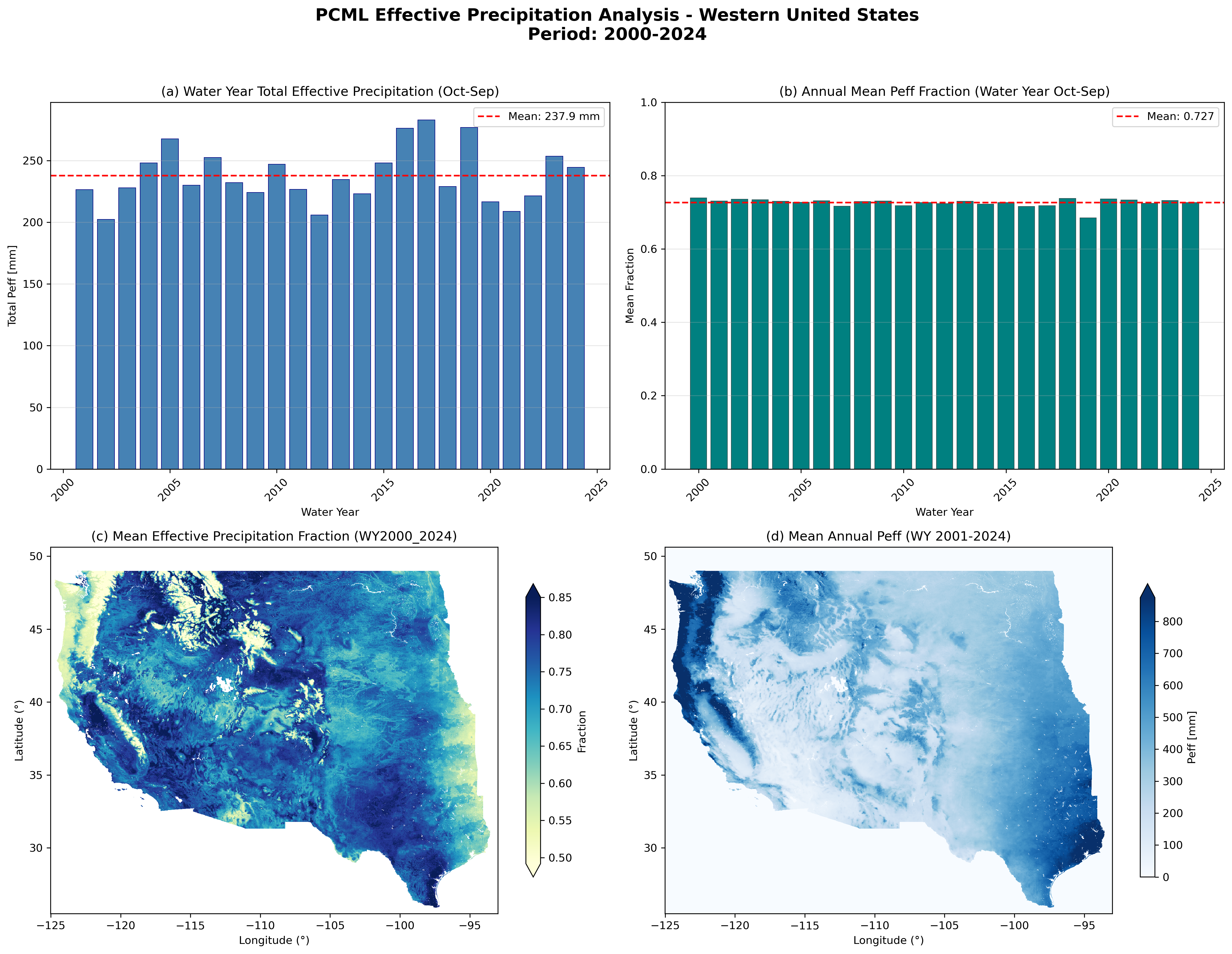
Summary of PCML effective precipitation analysis for the Western U.S. (WY 2001-2024): (a) Water year total time series, (b) Annual mean fraction time series, (c) Mean effective precipitation fraction map, (d) Mean annual effective precipitation map.
Mean Annual Effective Precipitation
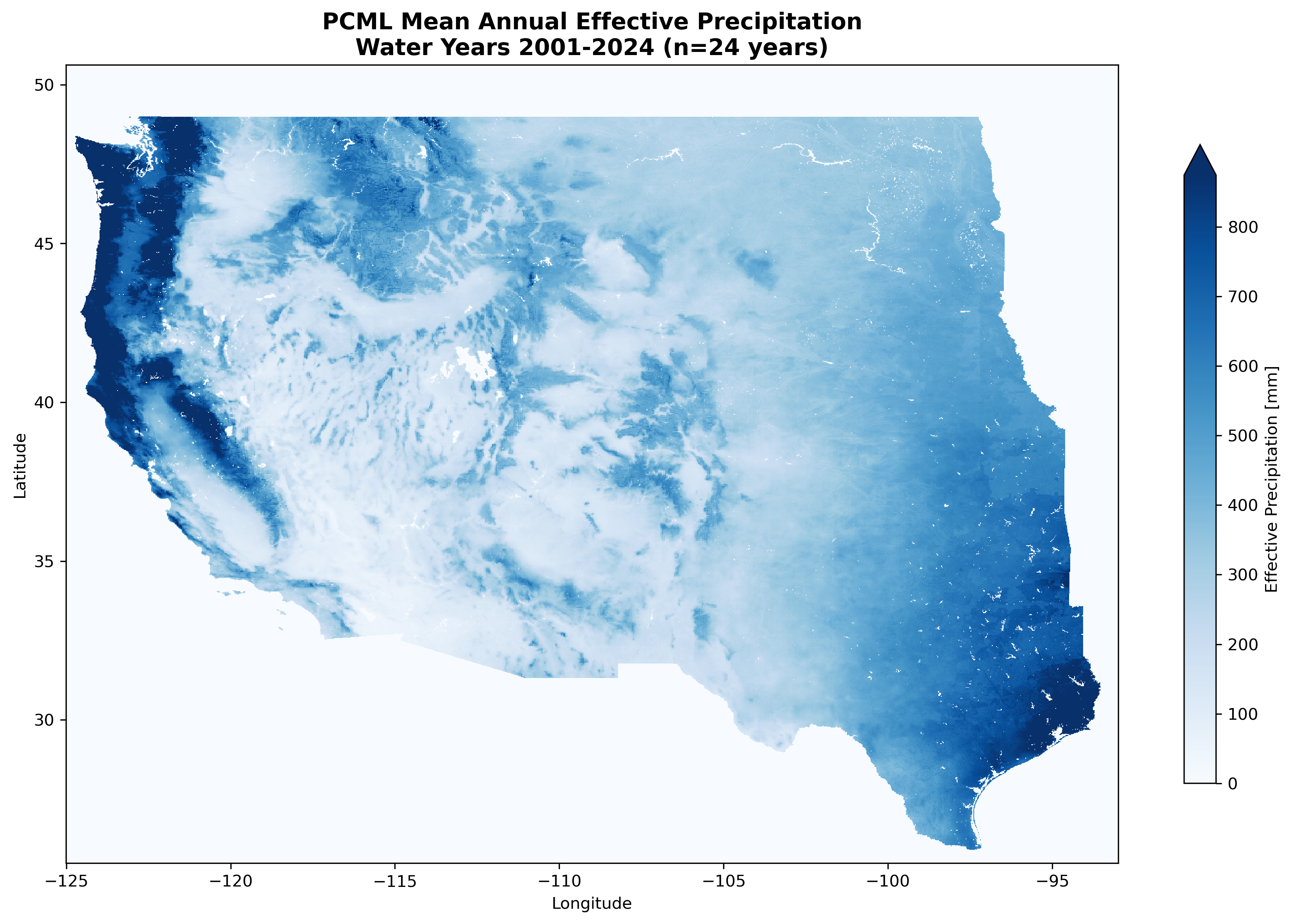
Mean annual effective precipitation (WY 2001-2024) for the Western United States computed from the PCML GEE asset.
Mean Effective Precipitation Fraction
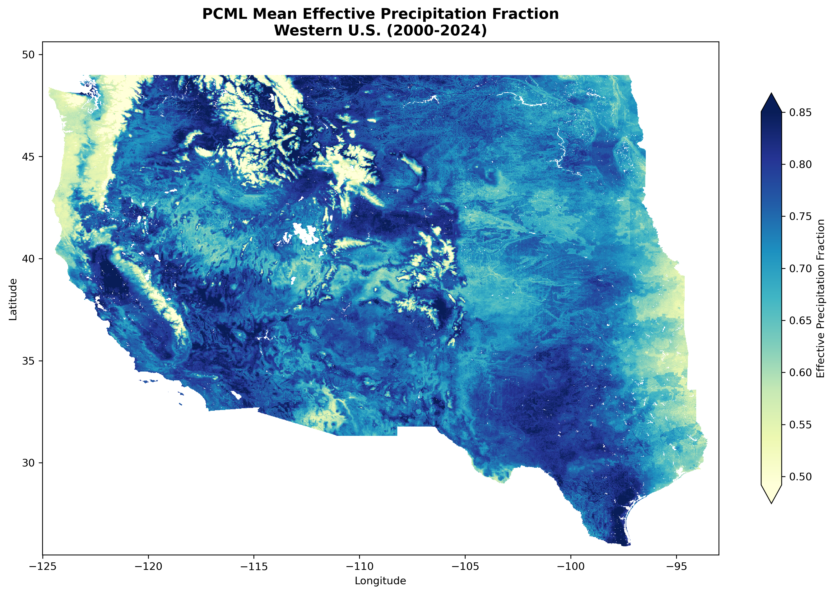
Mean annual effective precipitation fraction (Peff/Precip) for the Western United States (WY 2001-2024).
Reference: Hasan, M. F., Smith, R. G., Majumdar, S., Huntington, J. L., Alves Meira Neto, A., & Minor, B. A. (2025). Satellite data and physics-constrained machine learning for estimating effective precipitation in the Western United States and application for monitoring groundwater irrigation. Agricultural Water Management, 319, 109821.
Local Precipitation Examples (Your Own Files)
Since v1.3.0 pyCropWat can read monthly precipitation from disk instead of downloading it from Earth
Engine. Three ready-to-run scripts live in Examples/LocalPrecip/
(see Examples/LocalPrecip/README.md
for the full option list), and the Local Precipitation Data guide covers
the feature end-to-end.
| Script | Input | Method | Earth Engine |
|---|---|---|---|
local_precip_quickstart.py |
Directory of monthly GeoTIFFs | cropwat (any precipitation-only method) |
Not used |
wrf_south_america_local_example.py |
WRF South America GeoTIFFs + GEE AWC/ETo | usda_scs, then all 8 methods locally |
AWC and ETo only |
local_netcdf_example.py |
NetCDF stack built from the same GeoTIFFs | cropwat (any precipitation-only method) |
Not used |
All three expect the WRF South America example rasters at <repo>/../pyCropWat_Data/Precip, and all
three take --precip-dir to point at your own monthly rasters instead.
Local Precipitation Quick Start
The smallest possible local-data workflow: a directory of monthly rasters in, effective precipitation rasters out, with no Earth Engine involvement at all.
Ready-to-Run Script
Examples/LocalPrecip/local_precip_quickstart.py:
Defaults keep the first run small: --method cropwat, --start-year 2005 --end-year 2005,
--months 7 8, four workers, output in ./LocalPrecip_Quickstart.
Input Data
| Property | Value |
|---|---|
| Layout | One GeoTIFF per month, dated by file name (Precip_YYYY_MM.tif) |
| Units | Monthly totals; convert with precip_scale_factor if not already mm |
| Nodata | Read from the file metadata, plus any extra sentinel you pass (e.g. -9999) |
| CRS | Read from the file. local_precip_crs overrides it (and supplies one when the file declares none) - it relabels the grid, it never reprojects |
Recognised file-name layouts are YYYY_MM, YYYY-MM, YYYYMM and YYYY.MM. Anything else needs
local_precip_date_regex with named year and month groups.
Script Options
| Option | Default | Description |
|---|---|---|
--precip-dir |
<repo>/../pyCropWat_Data/Precip |
Directory of monthly precipitation GeoTIFFs |
--pattern |
Precip_*.tif |
Glob for the monthly rasters |
--nodata |
-9999.0 |
Extra nodata sentinel, on top of the file metadata |
--method |
cropwat |
Any precipitation-only method (cropwat, fao_aglw, fixed_percentage, dependable_rainfall, farmwest) |
--start-year / --end-year |
2005 / 2005 |
Period to process |
--months |
7 8 |
Months to process |
--output |
./LocalPrecip_Quickstart |
Output directory |
-w, --workers |
4 |
Parallel workers; 1 runs process_sequential() |
The script first opens the data with open_local_precipitation() and logs the resolved kind, file
count, month count, year range, CRS, grid shape, resolution and WGS84 bounds, then runs the
workflow and reports min/mean/max and the NaN count of the first output raster.
Python Example
from pycropwat import EffectivePrecipitation

ep = EffectivePrecipitation(
    local_precip='../pyCropWat_Data/Precip',
    local_precip_pattern='Precip_*.tif',
    local_precip_nodata=-9999,
    method='cropwat'
)

# start_year/end_year omitted -> inferred from the files (2000-2021 for this dataset)
results = ep.process(output_dir='./out_local_cropwat', n_workers=4)

for ep_path, epf_path in results[:3]:
    print(ep_path.name, epf_path.name)
CLI Example
pycropwat process \
    --local-precip ../pyCropWat_Data/Precip \
    --local-precip-pattern 'Precip_*.tif' \
    --local-precip-nodata -9999 \
    --method cropwat \
    --output ./out_local_cropwat
Key Features
- No Earth Engine:
ee.Initialize()is never called for precipitation-only methods, so the run works offline and without credentials - Automatic date range:
start_year/end_yearare inferred from the file names; a range you do supply is clamped to the years on disk (with a warning), and months with no file are skipped - Nodata preserved:
-9999pixels becomeNaNand stayNaNin both the effective precipitation and the fraction raster (they are not reported as a fraction of 0) - Same outputs as GEE runs:
effective_precip_YYYY_MM.tifandeffective_precip_fraction_YYYY_MM.tif, written on the input grid and CRS
Generated Outputs
LocalPrecip_Quickstart/
├── effective_precip_2005_07.tif
├── effective_precip_fraction_2005_07.tif
├── effective_precip_2005_08.tif
└── effective_precip_fraction_2005_08.tif
All downstream tooling (TemporalAggregator, StatisticalAnalyzer, Visualizer,
export_to_netcdf) works on these exactly as it does for GEE-derived outputs.
WRF South America Local Precipitation Example
This example runs the Rio de la Plata basin workflow from WRF regional climate model
precipitation stored on disk, while still pulling AWC and ETo from Earth Engine so that the
usda_scs and ensemble methods are available. It mirrors the two-step design of the GEE
examples: run USDA-SCS once with save_inputs=True, then calculate the remaining methods locally
from the saved precipitation, AWC and ETo rasters.
Ready-to-Run Script
Examples/LocalPrecip/wrf_south_america_local_example.py:
# Default period is 2000-2001 (24 months) so the first run is quick
python Examples/LocalPrecip/wrf_south_america_local_example.py

# The full WRF record
python Examples/LocalPrecip/wrf_south_america_local_example.py \
    --start-year 2000 --end-year 2021 -w 8
Other options: --precip-dir, --pattern, --nodata, --geometry (local vector file or GEE
FeatureCollection asset), --gee-project, --output (default ./WRF_SA_Local),
--download-only, --calc-only and -f/--force.
Local counterpart of the GEE WRF workflow
This is the local-file twin of
Examples/wrf/wrf_south_america_example.py,
which computes the same thing from the WRF precipitation GEE asset
(projects/azhydro/assets/WRF-ET-SA, band b1). Same domain, same period, same AWC/ETo assets,
same rooting depth and MAD factor, same output layout - the only difference is where the
precipitation comes from. Run both to compare a GEE-hosted ingestion against reading the
exported rasters directly.
WRF Precipitation Dataset
| Property | Value |
|---|---|
| Source | WRF regional climate model output, South America (Rio de la Plata basin domain) |
| Files | 264 monthly GeoTIFFs named Precip_YYYY_MM.tif |
| Period | January 2000 - December 2021 |
| CRS | EPSG:4326 |
| Grid | 689 rows x 799 columns at 0.0397 deg (~4.4 km) |
| Extent | 71.30°W - 39.54°W, 40.35°S - 12.96°S |
| Values | float32, already in millimetres per month (precip_scale_factor=1.0), nodata -9999 |
AWC and ETo (still from Earth Engine)
| Component | GEE Asset | Band | Scaling |
|---|---|---|---|
| AWC | projects/sat-io/open-datasets/FAO/HWSD_V2_SMU |
AWC |
awc_scale_factor=0.001 (mm/m → volumetric fraction) |
| ETo | IDAHO_EPSCOR/TERRACLIMATE |
pet |
eto_scale_factor=0.1, eto_is_daily=False |
Physical parameters: rooting_depth=2.0 m, mad_factor=1.0. Because AWC and ETo are downloaded,
this example does require Earth Engine credentials.
Methods Computed (8 total)
| # | Method | Inputs |
|---|---|---|
| 1 | USDA-SCS | Local precipitation + GEE AWC + GEE ETo |
| 2 | Ensemble | Mean of 6 methods, calculated locally |
| 3 | CROPWAT | Precipitation only |
| 4 | FAO/AGLW | Precipitation only |
| 5 | Fixed % (70%) | Precipitation only |
| 6 | Dependable Rainfall (75%) | Precipitation only |
| 7 | FarmWest | Precipitation only |
| 8 | TAGEM-SuET | Local precipitation + saved ETo |
PCML is excluded: it is a pre-computed Western U.S. GEE product and cannot be combined with local precipitation.
Python Example
from pycropwat import EffectivePrecipitation

ep = EffectivePrecipitation(
    local_precip='../pyCropWat_Data/Precip',
    local_precip_pattern='Precip_*.tif',
    local_precip_nodata=-9999,
    geometry_path=None,                 # optional: a vector file clips the local rasters
    start_year=2000,
    end_year=2001,
    precip_scale_factor=1.0,            # WRF rasters are already in mm
    gee_project='your-project-id',
    method='usda_scs',
    method_params={
        'awc_asset': 'projects/sat-io/open-datasets/FAO/HWSD_V2_SMU',
        'awc_band': 'AWC',
        'awc_scale_factor': 0.001,
        'eto_asset': 'IDAHO_EPSCOR/TERRACLIMATE',
        'eto_band': 'pet',
        'eto_scale_factor': 0.1,
        'eto_is_daily': False,
        'rooting_depth': 2.0,
        'mad_factor': 1.0
    }
)

# save_inputs writes precip_YYYY_MM.tif, awc.tif and eto_YYYY_MM.tif into input_dir
ep.process(
    output_dir='./WRF_SA_Local/usda_scs',
    input_dir='./WRF_SA_Local/analysis_inputs',
    n_workers=4,
    save_inputs=True
)
Step 2 of the script then reads those saved rasters back with rioxarray and applies the other
seven methods from pycropwat.methods - no further downloads required. Use --download-only to
stop after step 1, or --calc-only to re-run step 2 on inputs you already have.
CLI Example
pycropwat process \
    --local-precip ../pyCropWat_Data/Precip \
    --local-precip-pattern 'Precip_*.tif' \
    --local-precip-nodata -9999 \
    --start-year 2000 --end-year 2001 \
    --method usda_scs \
    --awc-asset projects/sat-io/open-datasets/FAO/HWSD_V2_SMU \
    --awc-band AWC --awc-scale-factor 0.001 \
    --eto-asset IDAHO_EPSCOR/TERRACLIMATE --eto-band pet --eto-scale-factor 0.1 \
    --rooting-depth 2.0 --mad-factor 1.0 \
    --project your-project-id \
    --workers 8 \
    --output ./WRF_SA_Local/usda_scs
ETo unit scaling
TerraClimate pet is stored in 0.1 mm units, so --eto-scale-factor 0.1 is required above.
Omitting it feeds USDA-SCS an ETo 10x too large and yields plausible-looking but wrong results.
GridMET and AgERA5 ETo are already in mm and keep the default 1.0. The Python API equivalent
is method_params={'eto_scale_factor': 0.1}.
Key Features
- Hybrid workflow: precipitation from disk, AWC and ETo from Earth Engine
- Grid alignment: GEE-sourced AWC and ETo are reprojected onto the local WRF grid, so the saved
awc.tif/eto_YYYY_MM.tifshare the transform and CRS ofprecip_YYYY_MM.tif - Native scale: the local grid resolution (~4.4 km) is used as the GEE download scale for AWC/ETo instead of the generic fallback
- Model-domain nodata: the WRF
-9999border is masked toNaNand stays masked in every output - Optional clipping:
--geometrywith a local vector file clips the monthly rasters; a GEE FeatureCollection asset ID is used for the AWC/ETo requests instead, leaving the rasters unclipped. Where the rasters are left unclipped, any pixel outside the AWC/ETo download region has no AWC or ETo to pair with, so it stays NaN in theusda_scs,ensembleandsuetoutputs and the run logs a WARNING naming the uncovered pixel count, once per field per process (twice forusda_scsandensemble: once for AWC, once for ETo) -AWC covers only 3.0% of the precipitation grid; 534255 pixel(s) will be NaN in the output. Clip the precipitation to the geometry (clip_to_geometry=True) or widen the geometry.Clip to the download region, or widen the geometry to span the whole grid, to get full coverage - Directly comparable to the GEE WRF example, which uses the same domain, period and parameters
Generated Outputs
WRF_SA_Local/
├── usda_scs/
│   ├── effective_precip_{year}_{month}.tif
│   └── effective_precip_fraction_{year}_{month}.tif
├── analysis_inputs/
│   ├── precip_{year}_{month}.tif      # the local WRF grid, as read (mm)
│   ├── awc.tif                        # HWSD AWC regridded to the WRF grid
│   └── eto_{year}_{month}.tif         # TerraClimate ETo regridded to the WRF grid
└── peff_by_method/                     # effective_precip_{year}_{month}.tif in each
    ├── usda_scs/
    ├── ensemble/
    ├── cropwat/
    ├── fao_aglw/
    ├── fixed_percentage/
    ├── dependable_rainfall/
    ├── farmwest/
    └── suet/
Local NetCDF Precipitation Example
pyCropWat reads local precipitation from NetCDF as easily as from a directory of GeoTIFFs. This example does the whole round trip and proves the two paths agree: it builds a NetCDF from the monthly WRF GeoTIFFs, computes effective precipitation from that NetCDF, recomputes the same months from the original GeoTIFFs, and asserts the two sets of rasters match. It uses a precipitation-only method, so no Earth Engine is involved.
Ready-to-Run Script
Examples/LocalPrecip/local_netcdf_example.py:
python Examples/LocalPrecip/local_netcdf_example.py
python Examples/LocalPrecip/local_netcdf_example.py --months 7 8      # quick run
python Examples/LocalPrecip/local_netcdf_example.py --skip-build      # reuse the .nc
Defaults: --year 2005, --method cropwat, --nodata -9999.0, all twelve months, output in
./LocalPrecip_NetCDF.
Workflow Steps
- Build
precip_YYYY.ncfrom the twelve monthly GeoTIFFs - variableprecip, dimensiontime(days since 1900-01-01),float32,_FillValue -9999, compressed whennetCDF4orh5netcdfis installed (thescipybackend is used as an uncompressed NetCDF3 fallback) - Inspect the file through
open_local_precipitation()and log kind, month count, year range, grid, CRS, bounds and the first month's mean - Compute effective precipitation from the NetCDF into
from_netcdf/ - Recompute the same months from the GeoTIFFs into
from_geotiff/and compare both rasters pixel-by-pixel (agreement within1e-4mm, with matching NaN masks, is asserted)
Input Data
| Property | Value |
|---|---|
| Layout | One or more .nc files; months come from the time coordinate, or from the file name when there is no time axis |
| Variable | Auto-detected (precip, precipitation, pr, prcp, ppt, tp, RAINNC, ...) or named with local_precip_variable |
| Dimensions | x/lon/longitude/west_east and y/lat/latitude/south_north are recognised automatically |
| CRS | Taken from the grid mapping when present. local_precip_crs overrides whatever the file declares (and supplies one when it declares none) - it relabels the grid, it never reprojects |
| Units | Monthly totals, converted with precip_scale_factor (e.g. 1000 for metres, 10 for centimetres, 25.4 for inches). A rate such as kg m⁻² s⁻¹ cannot be converted by any single multiplier, because the factor depends on the length of each month - accumulate to monthly totals first |
Python Example
from pycropwat import EffectivePrecipitation, open_local_precipitation

# Inspect the file first
with open_local_precipitation('./LocalPrecip_NetCDF/precip_2005.nc',
                              variable='precip',
                              nodata=-9999) as src:
    print(src.kind, len(src), src.year_range, src.crs, src.shape)
    print(src.available_months()[:3])

ep = EffectivePrecipitation(
    local_precip='./LocalPrecip_NetCDF/precip_2005.nc',
    local_precip_variable='precip',
    local_precip_nodata=-9999,
    method='cropwat'
)

results = ep.process(output_dir='./LocalPrecip_NetCDF/from_netcdf', n_workers=4)
A multi-file stack works the same way - pass a directory with local_precip_pattern='*.nc', or a
glob such as './netcdf/precip_*.nc'. Add local_precip_crs='EPSG:4326' when the file declares no
CRS, or to override one it declares wrongly - the grid is relabelled in place, never reprojected.
CLI Example
pycropwat process \
    --local-precip ./LocalPrecip_NetCDF/precip_2005.nc \
    --local-precip-variable precip \
    --local-precip-nodata -9999 \
    --method cropwat \
    --output ./LocalPrecip_NetCDF/from_netcdf
Add --local-precip-crs EPSG:4326 for a file that carries no CRS, or to override one it declares
wrongly. The flag relabels the grid; it never reprojects it.
Key Features
- Time-axis aware: months are read from the NetCDF
timecoordinate (standard andcftimecalendars), falling back to file-name dating when there is no usable time axis - Variable auto-detection: common precipitation variable names are found automatically; an
ambiguous file raises a
ValueErrornaming the candidates - Flexible grids: non-standard dimension names are recognised, 1-D coordinates are derived from 2-D curvilinear coordinates when needed, and south-up grids are flipped to north-up
- Thread-safe reads: NetCDF handles are shared, so reads are serialised with a lock while the
parallel
process()path fans months out across Dask threads _FillValue/missing_valuehonoured, plus any extralocal_precip_nodatasentinel- Verified equivalence: the script asserts the NetCDF and GeoTIFF results agree to within
1e-4mm, exiting non-zero if they do not